If you launch a projectile and let it move ballistically – under uniform gravity, in the absence of air resistance – its trajectory will be a parabola (or a straight line, if you launch it straight upwards). If you were a passenger in such a projectile, you would be weightless while it was in flight.
But suppose that you equipped the projectile with a rocket that fired with a constant thrust, always perpendicular to the direction the projectile was moving, and always in the same plane. Neglecting any change in the mass of the projectile as it used up fuel (and again neglecting air resistance), it would be subject to both ordinary gravitational acceleration towards the ground, and a constant perpendicular acceleration due to the rocket. In this case, a passenger would feel as if their weight was constant, at a value determined by the thrust from the rocket.
The trajectory of such a projectile would no longer be a parabola, and the exact shape would depend on the launch velocity and the amount of perpendicular acceleration. But once we know the trajectory, this leads to another possibility: rather than providing the perpendicular force with a rocket, the same effect could be achieved if we built a rollercoaster whose track was shaped to mimic the same curve. The force exerted by a rollercoaster track on a car sliding along it (neglecting friction) will always be perpendicular to the car’s direction of motion, so by matching the trajectory of a projectile with constant perpendicular acceleration, we can build a rollercoaster whose passengers experience a constant weight (either less than, or greater than, their ordinary weight), for the duration of their trip.
The acceleration for the projectile we have described will be given by:
a = (ax, az) = (α/v)(–vz, vx) + (0, –g)
where α is the constant perpendicular acceleration due to the rocket (or the normal force from the rollercoaster track), v=√(vx2 + vz2) is the current speed of the projectile or rollercoaster car, and g is the acceleration due to gravity.
However, before we go ahead and solve for this particular case, we will write a slightly more general form, where the magnitude of the perpendicular acceleration might not actually be constant, but can depend in some fashion on the speed, v:
a = (ax, az) = (α(v)/v)(–vz, vx) + (0, –g)
One well-known case where α(v) is not constant but takes a very simple form is the Lorentz force experienced by a charged particle in a constant magnetic field. We have:
FLorentz = q v × B
where q is the charge of the particle and B is the magnetic field vector. For our purposes, we will suppose that B is a constant vector pointing in the y direction, B = B ey, and we can accommodate the Lorentz force by setting:
α(v) = ω v
ω = q B / m
Here ω is the angular cyclotron frequency, which gives the rate at which a [non-relativistic particle] of mass m and charge q would move around in a circle, if it was subject only to a magnetic field of strength B. In our scenario, we are complicating that by effectively tipping the cyclotron onto its side and adding gravitational acceleration in the same plane as the usual circular motion.
In order to proceed, we will start by noting that when α(v) = 0 and the trajectory is a parabola, the horizontal velocity of the projectile, vx, remains constant. In general, we don’t expect vx to be constant, but we will write down a new quantity, C(v), that depends only on vx and the overall speed, v:
C(v) = g vx – f(v)
and see if we can find a relationship between f(v) and α(v) that makes C(v) constant.
From our general formula for the acceleration a, we obtain two useful results:
a · v = –g vz
ax = –(α(v)/v) vz
We can write the rate of change of C(v) with time as:
dC(v) / dt = g ax – df(v) / dt
= g ax – f '(v) d(√(v · v)) / dt
= g ax – f '(v) a · v / (√(v · v))
= (g vz / v) (f '(v) – α(v))
So we can make C(v) a constant of the motion if we have:
f '(v) = α(v)
For our original case of the projectile with constant perpendicular acceleration α:
α(v) = α
f(v) = α v
C(v) = g vx – α v
For the cyclotron, where the acceleration is a linear function of the particle’s speed:
α(v) = ω v
f(v) = ½ ω v2
C(v) = g vx – ½ ω v2
As well as C(v) being conserved, the total energy of the projectile, kinetic energy plus potential energy, will also remain constant. This is because the perpendicular force, being orthogonal to the velocity of the projectile, doesn’t alter its kinetic energy; only gravity does that, and the change in kinetic energy due to gravity will always be balanced by an opposite change in gravitational potential energy.
If we assume that the projectile was launched from a height of z0 with a speed of v0 at an angle of θ to the horizontal, we can use conservation of energy to obtain a simple relationship between the projectile’s height and its speed:
½ v2 + g z = ½ v02 + g z0
v2 = v02 – 2 g (z – z0)
For the sake of simplicity, we will set z0 = 0, and then we have:
v(z) = √(v02 – 2 g z)
To obtain the shape of the trajectory, we can start with:
dx/dz = vx / vz
= vx / √(v2 – vx2)
= vx / √(v02 – 2 g z – vx2)
We can obtain vx in terms of z from the conservation of C(v). For the projectile / rollercoaster, we have:
g vx – α v = g v0 cos θ – α v0
g vx – α √(v02 – 2 g z) = g v0 cos θ – α v0
vx = v0 cos θ + (α/g) (√(v02 – 2 g z) – v0)
For convenience, we will define β = α/g, in order to make some formulas for the rollercoaster curves more concise.
For the tipped-over cyclotron we have:
g vx – ½ ω v2 = g v0 cos θ – ½ ω v02
g vx – ½ ω (v02 – 2 g z) = g v0 cos θ – ½ ω v02
vx = v0 cos θ – ω z
In both cases, we can integrate dx/dz to obtain explicit expressions for x(z), though they are quite complicated.
For the projectile / rollercoaster, the solution is:
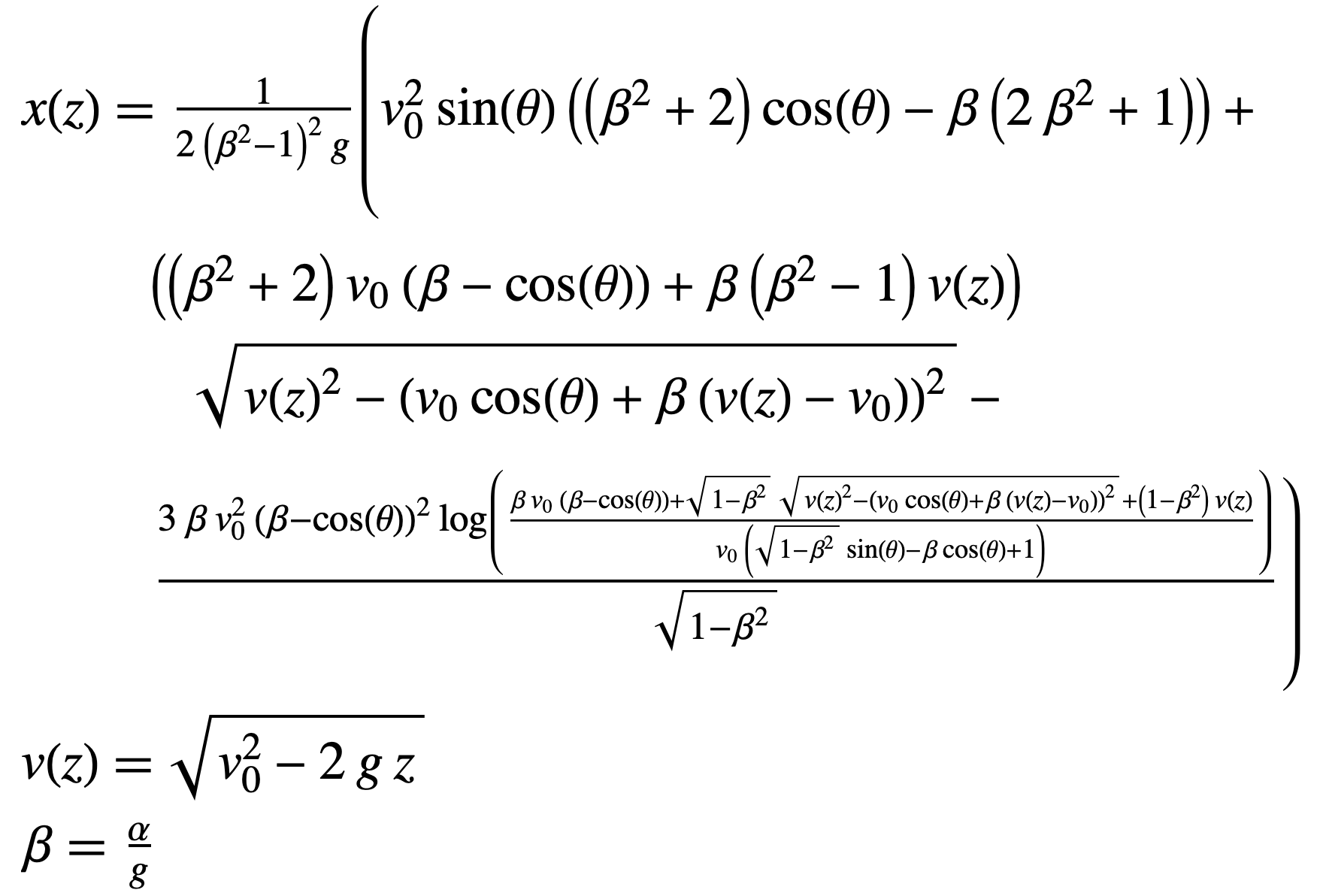
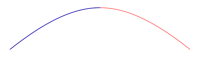
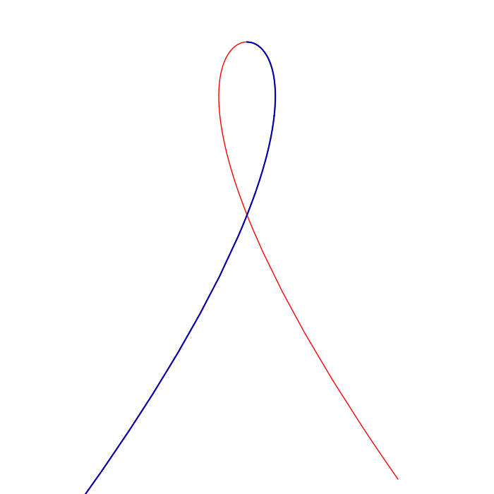
This formula will only give part of the trajectory, because x will take more than one value for a given z, but we can extend the basic shape we get this way by reflecting, and in some cases repeating, the initial segment. In the plots below, the formula gives us the blue part of the curve, but it’s easy to see how that shape is reused to make the whole trajectory.
 |
 |
 |
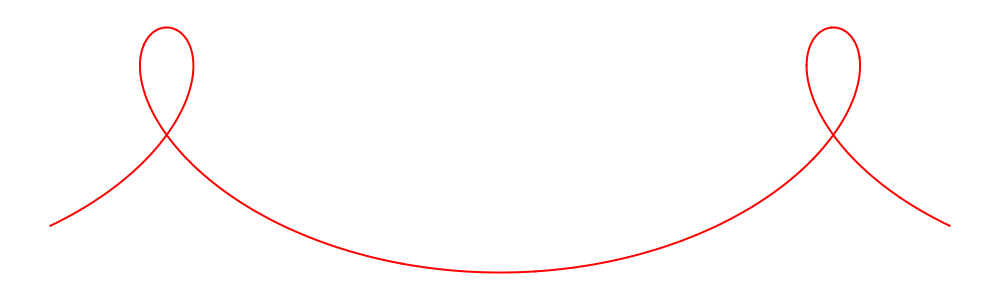
| β = 1/2, v0 = 20 and θ = 0 0 < β < cos θ C > 0 |
β = 0.95, v0 = 20 and θ = π/3 cos θ < β < 1 C < 0 |
β = 2, v0 = 20 and θ = 0 β > 1 C < 0 |
Although the trajectory for β = 1/2 looks a bit like a hyperbola, and the trajectory for β = 2 looks a bit like a prolate trochoid, the actual shapes are different.
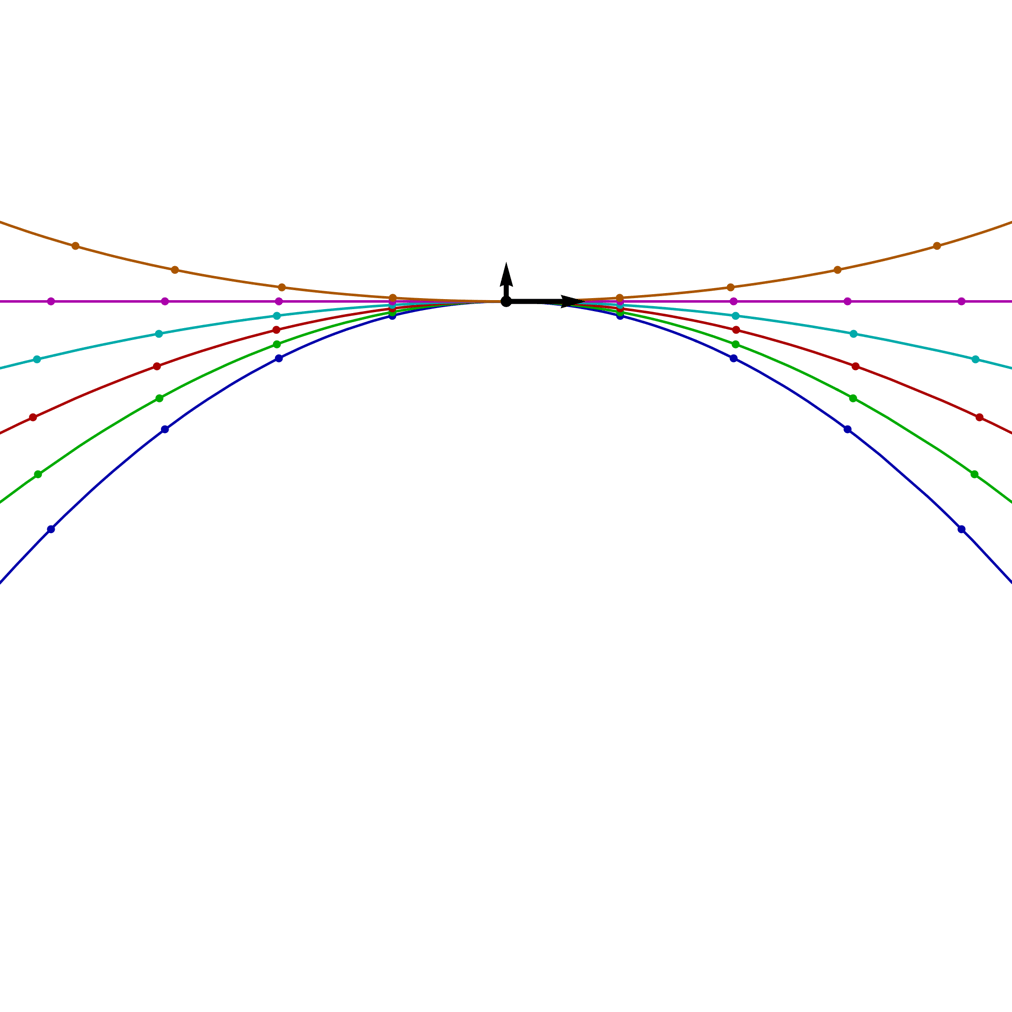
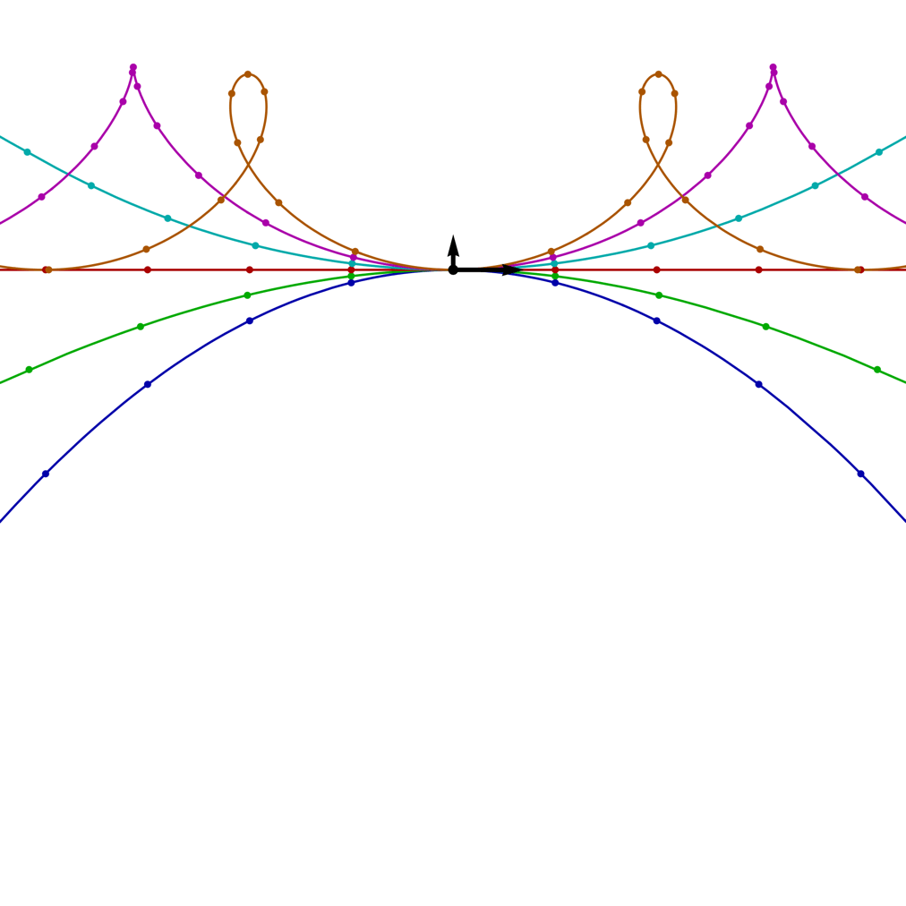
The image on the left shows the trajectories for projectiles with a range of β values (blue = 0, 1/4, 1/2, 3/4, 1, orange = 5/4) and a fixed launch speed v0 = 20, as the launch angle θ rotates through a full circle. The arrows show the initial direction of the velocity and the perpendicular force; the small circles on the trajectories mark the positions of the projectile at equally spaced time intervals.
If β is less than cos θ, the trajectory contains no loops and resembles a hyperbola, as with the example above for β = 1/2. This criterion might seem a bit strange, since the angle of the trajectory changes over time, so merely by calling different moments in time the “launch” of the projectile, we can have different values for θ.
However, the quantity C(v) = g vx – α v = g v (cos θ – β) is conserved, and since the sign of v cannot be negative, the sign of cos θ – β cannot change. So for trajectories of this kind, the range of θ is restricted to –arccos(β) < θ < arccos(β). And, although the curve is not a hyperbola, like a hyperbola it will be asymptotic to two straight lines, at angles θ = ±arccos(β).
When β = cos θ, the trajectory is simply a straight line, because the perpendicular force is the same as that provided by an inclined plane at an angle of θ.
For values of β that are less than 1, but greater than cos θ, the trajectory contains a single loop at its highest point, but still falls infinitely low on either side, as with the example for β = 0.95. Again, this criterion holds throughout the trajectory: although the projectile completes a loop, its velocity doesn’t swing around through a complete circle, and as it moves between two asymptotic lines at θ = ±arccos(β) the condition on cos θ continues to hold.
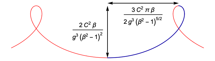
For values of β greater than 1, the trajectory is spatially periodic, containing multiple loops, and it never falls below a certain height, as with the example above for β = 2. We can compute the distance between the highest and lowest heights in the trajectory in terms of the invariant C, by noting that these extrema occur when cos θ = ±1, and so v = C/[g(±1 – β)].
Solving for z in the equation v = √(v02 – 2 g z) and taking the difference between the two values, we get:
Δz = 2 C2 β / [g3 (β2 – 1)2]
If we plug the same values for z into our solution for x(z), we find that:
Δx = 3 C2 π β / [2 g3 (β2 – 1)5/2]
The ratio is independent of C:
Δx/Δz = 3 π / [4 √(β2 – 1)]
In fact, while C2 / g3 sets the overall scale of the trajectory, and the sign of C determines whether or not loops are present, in all other respects the shape of the trajectory is determined by β, and is independent of C.
For the tipped-over cyclotron, the solution is:

As with the rollercoaster solution, this formula will only give part of the trajectory, because x will take more than one value for a given z. We can obtain the whole trajectory by reflecting and repeating this initial segment.
 |
 |
 |
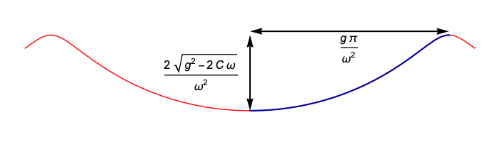
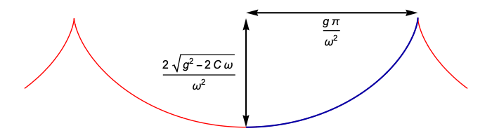
| ω = 4/5, v0 = 20 and θ = 0 C > 0 |
ω = 1, v0 = 20 and θ = 0 C = 0 |
ω = 5/4, v0 = 20 and θ = 0 C < 0 |
The image on the right shows the trajectories for a tipped-over cyclotron with a range of ω values (blue = 0, 1/4, 1/2, 3/4, 1, orange = 5/4) and a fixed launch speed v0 = 20, as the launch angle θ rotates through a full circle. The arrows show the initial direction of the velocity and the perpendicular force; the small circles on the trajectories mark the positions of the projectile at equally space time intervals.
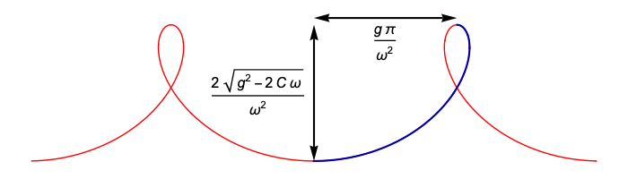
In this case, the resemblance to trochoids is not misleading! These trajectories are precisely what you get from rolling a circle of radius r = g/ω2 along a horizontal line (with the circle below the line), while tracing out the path of a point attached to the circle, at a distance of R = √(g2–2Cω)/ω2 from the centre of the circle.
Here, C is the tipped-over cyclotron conserved quantity:
C(v) = g vx – ½ ω v2
Specifically, the trajectory is:
This picture of a curve traced out by a point attached to a rolling circle doesn’t just give the correct shape of the trajectory, it also matches the motion of the particle over time.
With a suitable choice of origin, for a circle of radius r rolling with angular frequency ω, the coordinates of a point attached to the circle at a distance of R from its centre are:
x(t) = r ω t – R sin ω t
z(t) = R cos ω t
It follows that the velocities and accelerations are:
vx(t) = r ω – ω R cos ω t
vz(t) = –ω R sin ω t
ax(t) = ω2 R sin ω t
az(t) = –ω2 R cos ω t
Inserting these results into the relationship between velocity and acceleration for the tipped-over cyclotron, we get:
(ax, az) = ω (–vz, vx) + (0, –g)
(ω2 R sin ω t, –ω2 R cos ω t) = (ω2 R sin ω t, r ω2 – ω2 R cos ω t – g)
So this relationship will hold true so long as we set r = g/ω2. And for the conserved quantity C, we have:
C = g vx – ½ ω v2
= g [r ω – ω R cos ω t] – ½ ω [(r ω – ω R cos ω t)2 + (–ω R sin ω t)2]
= g [r ω – ω R cos ω t] – ½ ω [r2 ω2 – 2 ω2 R r cos ω t + ω2 R2]
= ω R [ω2 r – g] cos ω t + [g r ω – ½ ω3 (R2 + r2) ]
This will only be constant if we set r = g/ω2, in which case it becomes:
C = g2/ω – ½ ω3 (R2 + g2/ω4)
2 C = g2/ω – ω3 R2
R2 = (g2–2Cω)/ω4
giving us the original value we claimed for R.
We have seen that the motion of a particle subject to the acceleration:
a = (ax, az) = (f '(v)/v)(–vz, vx) + (0, –g)
possesses a conserved quantity:
C(v) = g vx – f(v)
where f(v) is any differentiable function of the particle’s speed v. We have already proved this directly, with a simple calculation, so in a sense there is nothing at all mysterious about it.
But a question remains:
Does this conserved quantity arise from some kind of symmetry?
The connection between symmetries and conserved quantities in physical systems is encapsulated by Noether’s theorem. This is phrased in the language of Lagrangian mechanics, so we will start with a quick overview of that subject, largely following [1].
Many physical systems can be described by laws of motion that can be obtained by requiring the trajectory of the system to yield an extreme value (either a maximum or a minimum) for the integral over time of a certain quantity, when compared to all the other trajectories that start and end at the same points in space.
For example, the trajectory that a projectile follows, when moving under uniform gravity, given that it starts at point (x1, z1) at time t1 and arrives at point (x2, z2) at time t2, will be the one that minimises the integral:
S = ∫t1t2 ½ m (vx(t)2 + vz(t)2) – g m z(t) dt
The quantity we integrate here is called the Langrangian of the system, ℒ, and the integral S is known as the action.
The ultimate reason why this condition holds lies in quantum mechanics, where each path a particle can take is given a phase that depends on the action, and if the action for some path is a local maximum or minimum, the paths very close to it are all in phase, and so they reinforce each other rather than cancelling out. But for our purposes, we will just take it as given that some purely classical laws of motion can be produced this way. And some can’t, but we will have more to say about that later.
The Lagrangian ℒ will generally be a function of several coordinates x(t), y(t), z(t), ..., the rates of change of those coordinates (aka velocities), vx(t), vy(t), vz(t), ..., and it might also have an explicit dependence on time, t. Then the action is:
S = ∫t1t2 ℒ (x(t), y(t), z(t), ..., vx(t), vy(t), vz(t), ..., t) dt
Now, suppose we pick a differentiable function δ(t) that satisfies:
δ(t1) = 0
δ(t2) = 0
and consider the value the action S takes if we add some multiple of δ(t) to, say, the x coordinate:
S(ε) = ∫t1t2 ℒ (x(t) + ε δ(t), y(t), z(t), ..., vx(t) + ε δ'(t), vy(t), vz(t), ..., t) dt
The derivative of this with respect to ε is:
dS(ε)/dε = ∫t1t2 (∂ℒ /∂x) δ(t) + (∂ℒ /∂vx) δ'(t) dt
We can use integration by parts on the second term, and the fact that δ is zero on the endpoints of the range of integration, to convert this to:
dS(ε)/dε = ∫t1t2 [(∂ℒ /∂x) – d/dt (∂ℒ /∂vx)] δ(t) dt
Since our original S has a local extremum amongst all suitable trajectories, the rate of change of S(ε) with respect to ε must be zero at ε = 0, and this must be true for any choice of δ that meets the conditions on the endpoints. What’s more, the same must be true if we add δ to any one of the coordinates. So, for each coordinate x, y, z, ... an equation like the following must hold:
d/dt (∂ℒ /∂vx) = ∂ℒ /∂x
These are known as the Euler-Lagrange equations, and they will be true when the coordinates are functions of time that yield a local extreme value for the action.
To be clear, what we mean here by d/dt of an expression that might depend explicitly on t, but also on the coordinates and/or velocities, is that we use the chain rule, adding up the product of each of the partial derivatives of the expression with respect to those variables, with the derivative of each variable with respect to time. Since the derivative of a coordinate with respect to time is a velocity, and the derivative of a velocity with respect to time is an acceleration, we have:
d/dt f(x(t), y(t), ..., vx(t), vy(t), ..., t) = vx(t) ∂f/∂x + vy(t) ∂f/∂x + ... + ax(t) ∂f/∂vx + ay(t) ∂f/∂vy + ... + ∂f/∂t
To give a simple example, suppose we have:
ℒ (z, vx, vz) = ½ m (vx(t)2 + vz(t)2) – g m z(t)
This is the Lagrangian for a particle moving in two dimensions, with a uniform gravitational acceleration of g. It has no explicit dependence on either time t or the x coordinate. The Euler-Lagrange equations for this system are, for the x coordinate:
d/dt (∂ℒ /∂vx) = ∂ℒ /∂x
d/dt (m vx(t)) = 0
m ax(t) = 0
and for the z coordinate:
d/dt (∂ℒ /∂vz) = ∂ℒ /∂z
d/dt (m vz(t)) = –g m
m az(t) = –g m
In other words, the particle has zero acceleration, and hence a constant velocity, in the x direction, and an acceleration of –g in the z direction. We could have just written down these equations straight away, but the fact that we can obtain them from the Euler-Lagrange equations tells us that we have chosen the correct Lagrangian for this system.
It’s not hard to show that for any potential energy U(x, y, z), setting the Lagrangian equal to the difference between the kinetic and potential energy:
ℒ (x, y, z, vx, vy, vz) = ½ m (vx(t)2 + vy(t)2 + vz(t)2) – U(x(t), y(t), z(t))
will yield Euler-Lagrange equations that can be summed up in the vector equation:
m a(t) = –∇U(x(t), y(t), z(t))
which just amounts to saying that, for this system, the force on a particle is equal to the opposite of the gradient of its potential energy.
The Lagrangian is not unique! If we multiply a Lagrangian by any non-zero constant, it will yield exactly the same equations of motion, since the constant will appear on both sides of the Euler-Lagrange equations. But we can go much further than that. Suppose we have:
ℒ2 = ℒ1 + d/dt F(x(t), y(t), ..., t)
where F is any differentiable function of the coordinates and time (but not the velocities). The new action associated with this Lagrangian will then be:
S2 = ∫t1t2 ℒ2 dt = S1 + F(x(t2), y(t2), ..., t2) – F(x(t1), y(t1), ..., t1)
The last two terms here will be completely unchanged by adding the variation ε δ(t) to any of the coordinates, given that δ is zero at the endpoints t1 and t2. So if we use ℒ2 instead of ℒ1, we will again end up with exactly the same equations of motion.
We are interested in Lagrangians primarily for what they have to tell us about symmetries and conserved quantities, and our example of a particle moving under uniform gravity already offers a simple illustration of this. The fact that the Lagrangian:
ℒ (z, vx, vz) = ½ m (vx(t)2 + vz(t)2) – g m z(t)
has no dependence on x is an example of a symmetry: the Lagrangian is unchanged if we add a constant value to the x coordinate of a particle’s trajectory. Associated with that symmetry is a conserved quantity. From the Euler-Lagrange equation:
d/dt (∂ℒ /∂vx) = ∂ℒ /∂x
we see that the symmetry makes the RHS, ∂ℒ /∂x, equal to zero, which in turn makes the expression we are taking the time derivative of, ∂ℒ /∂vx, a constant. So we have:
∂ℒ /∂vx = m vx(t) = constant
In other words, the x component of the particle’s momentum is conserved.
At this point, we need to say something about the word momentum. In Newtonian physics, the momentum of a particle is just the product of its mass and its velocity:
p = m v
But in Lagrangian and Hamiltonian mechanics, the word has another meaning (even though the two meanings will coincide for certain systems). The Hamiltonian momentum “conjugate to” a coordinate such as x is defined as:
px = ∂ℒ /∂vx
This will agree with the Newtonian momentum if the only dependence of the Lagrangian on the velocity vx is due to an ordinary kinetic energy term, as is true for our particle moving under uniform gravity. But in some other systems, this will not be the case.
So: if a coordinate does not appear in the Lagrangian, then increasing that coordinate by some constant amount is a symmetry of the Lagrangian, and associated with that symmetry, we have the fact that the momentum conjugate to the coordinate is conserved.
But what if we did something more elaborate to the trajectory of the system, and the Lagrangian either remained unchanged, or was changed in a way that left the Euler-Lagrange equations unchanged? Suppose that, instead of moving our trajectory by a constant amount in a single coordinate direction, we moved it in a way such that the rate of change of each coordinate was some general function of the coordinates.
We will introduce a parameter s that describes how far we have moved the trajectory. Then for three coordinates, say, x, y, z, we will have something like:
∂x/∂s = Sx(x(t), y(t), z(t))
∂y/∂s = Sy(x(t), y(t), z(t))
∂z/∂s = Sz(x(t), y(t), z(t))
Since the coordinates change over time, any given trajectory will generally be subject to different displacements throughout its history. Unlike a simple translation, where we just slide everything along by a fixed amount in a constant direction, trajectories can change their orientation and their shape under this kind of flow. If we account for the change in velocities this produces, as well as the change in coordinates, we find that:
∂ℒ /∂s = Sx(x, y, z) ∂ℒ /∂x + Sy(x, y, z) ∂ℒ /∂y + Sz(x, y, z) ∂ℒ /∂z +
(vx ∂Sx/∂x + vy ∂Sx/∂y + vz ∂Sx/∂z) ∂ℒ /∂vx +
(vx ∂Sy/∂x + vy ∂Sy/∂y + vz ∂Sy/∂z) ∂ℒ /∂vy +
(vx ∂Sz/∂x + vy ∂Sz/∂y + vz ∂Sz/∂z) ∂ℒ /∂vz
That looks a bit daunting, so consider this example, which amounts to rotating the coordinates in the xy plane around the origin:
Sx(x, y, z) = y
Sy(x, y, z) = –x
Sz(x, y, z) = 0
Suppose we have a Lagrangian that is invariant under this flow. That means it will satisfy the equation:
∂ℒ /∂s = y ∂ℒ /∂x – x ∂ℒ /∂y + vy ∂ℒ /∂vx – vx ∂ℒ /∂vy = 0
As an example of a Lagrangian with this symmetry, consider the gravitational potential U(r) = –m k/r, which in Cartesian coordinates gives us:
ℒ (x, y, z, vx, vy, vz) = ½ m (vx(t)2 + vy(t)2 + vz(t)2) + m k / √(x(t)2+y(t)2+z(t)2)
How do we find the conserved quantity associated with a more complicated symmetry like this? We will take a guess and compute the rate of change of a candidate:
CS = Sx px + Sy py + Sz pz
In the following calculation, remember that px means ∂ℒ /∂vx by definition, and the Euler-Lagrange equations give us dpx/dt = ∂ℒ /∂x etc.
dCS / dt
= d/dt (Sx px + Sy py + Sz pz)
= Sx dpx/dt + dSx/dt px + Sy dpy/dt + dSy/dt py + Sz dpz/dt + dSz/dt pz
= Sx ∂ℒ /∂x + Sy ∂ℒ /∂y + Sz ∂ℒ /∂z +
(vx ∂Sx/∂x + vy ∂Sx/∂y + vz ∂Sx/∂z) ∂ℒ /∂vx +
(vx ∂Sy/∂x + vy ∂Sy/∂y + vz ∂Sy/∂z) ∂ℒ /∂vy +
(vx ∂Sz/∂x + vy ∂Sz/∂y + vz ∂Sz/∂z) ∂ℒ /∂vz
= ∂ℒ /∂s
When the Lagrangian is invariant under the flow described by S this is zero, and CS will be conserved.
For our example of a rotation in the xy plane, the conserved quantity is:
Sx px + Sy py + Sz pz = y px – x py
which is the z component of the angular momentum vector. The conservation of the other two components of the angular momentum vector can be shown to arise in exactly the same way from the invariance of the Lagrangian under rotations in the other two planes.
But what if the Lagrangian itself is not invariant under the flow, but changes by a time derivative of some function of the coordinates and time:
∂ℒ /∂s = d/dt F(x(t), y(t), z(t), t)
We can still construct a conserved quantity. Define:
CS, F = Sx px + Sy py + Sz pz – F(x(t), y(t), z(t), t)
Then we have:
dCS, F / dt = dCS / dt – d/dt F(x(t), y(t), z(t), t)
= ∂ℒ /∂s – d/dt F(x(t), y(t), z(t), t)
= 0
We can describe the tipped-over cyclotron with a fairly simple Lagrangian. Note that we could multiply everything here by the mass of the particle, m, to give the usual forms for the kinetic energy and the gravitational potential energy, but since m is a constant it would make no difference, so we will omit it.
ℒ (x, z, vx, vz) = ½ (vx(t)2 + vz(t)2) – g z(t) – ½ ω (x(t) vz(t) – z(t) vx(t))
The Hamiltonian momenta for the x and z coordinates are:
px = ∂ℒ /∂vx = vx(t) + ½ ω z(t)
pz = ∂ℒ /∂vz = vz(t) – ½ ω x(t)
and the Euler-Lagrange equations give us:
dpx/dt = ∂ℒ /∂x
ax(t) + ½ ω vz(t) = –½ ω vz(t)
ax(t) = –ω vz(t)
dpz/dt = ∂ℒ /∂z
az(t) – ½ ω vx(t) = ½ ω vx(t) – g
az(t) = ω vx(t) – g
These are the accelerations for the tipped-over cyclotron, confirming that the Lagrangian we have given is correct.
To find a conserved quantity for this system, we don’t need any kind of elaborate flow; we can just look at what happens if we shift the trajectory by a constant amount in the x direction. We have:
∂ℒ /∂x = –½ ω vz(t)
The Langrangian is not translation-invariant in the x direction, but its rate of change is a time derivative:
∂ℒ /∂x = d/dt (–½ ω z(t))
It follows from the results of the previous section that we can define a conserved quantity:
Cx = px + ½ ω z
= vx + ω z
If the trajectory is the trochoid:
x(t) = r ω t – R sin ω t
z(t) = z0 + R cos ω t
then this conserved quantity gives us:
Cx = vx + ω z = ω (z0 + r)
which is ω times the z coordinate of the horizontal line that the circle of radius r rolls along.
Of course, this is not the quantity we found initially:
C(v) = g vx – ½ ω v2
However, if we note that we have a conserved specific energy (energy per unit mass) for this system:
E = ½ v2 + g z
we can recover C(v) as:
C(v) = g Cx – ω E
Another way to obtain Cx is to change the Lagrangian, by adding a time derivative to it that removes its dependence on x. Adding a time derivative of a function of the coordinates to the Lagrangian has no effect on the equations of motions, so we can define:
ℒ0(z, vx, vz) = ℒ (x, z, vx, vz) + ½ ω d/dt (x(t) z(t))
= ℒ (x, z, vx, vz) + ½ ω (x(t) vz(t) + z(t) vx(t))
= ½ (vx(t)2 + vz(t)2) – g z(t) + ω z(t) vx(t)
(Thanks to Zach McDargh for pointing out this transformation.)
We now have:
px = ∂ℒ0/∂vx = vx(t) + ω z(t) = Cx
dpx/dt = ∂ℒ0/∂x = 0
Can the equations of motion for the constant-weight rollercoaster be produced by a Lagrangian?
The inverse Lagrangian problem, which seeks to find a Lagrangian whose Euler-Lagrange equations correspond to some specified set of ordinary differential equations (in our case, those that describe the known accelerations), is notoriously difficult. In 1941, Jesse Douglas published a complete analysis[2] for the case of two coordinates; in effect, he gave an algorithm that will either result in the desired Lagrangian, or in a definitive conclusion that no such function exists.
For the constant-weight rollercoaster, the verdict is: no such Lagrangian exists.
Douglas’s algorithm is quite complicated, so we won’t go through the calculations. But as a kind of consolation prize, his method does produce a Lagrangian for the version where we set g=0, i.e. when we have acceleration of constant magnitude α that is orthogonal to the velocity of a particle moving in a plane, with no additional forces:
a = (ax, az) = (α/v)(–vz, vx)
Clearly the solution to the equations of motion in this case is for the particle to move in a circle at a constant speed.
The Lagrangian obtained by applying Douglas’s algorithm is:
ℒ (x, z, vx, vz) = ⅓ (vx2 + vz2)3/2 + (α/2)(z vx – x vz)
The Hamiltonian momenta for the x and z coordinates are:
px = ∂ℒ /∂vx = vx v + (α/2) z
pz = ∂ℒ /∂vz = vz v – (α/2) x
and the Euler-Lagrange equations give us:
dpx/dt = ∂ℒ /∂x
[(2 vx2 + vz2) / v] ax + [vx vz / v] az + (α/2) vz = –(α/2) vz
[(2 vx2 + vz2) / v] ax + [vx vz / v] az + α vz = 0
dpz/dt = ∂ℒ /∂z
[(2 vz2 + vx2) / v] az + [vx vz / v] ax – (α/2) vx = (α/2) vx
[(2 vz2 + vx2) / v] az + [vx vz / v] ax – α vx = 0
These equations are solved by the accelerations we specified above.
Since ∂ℒ /∂x and ∂ℒ /∂z are both time derivatives:
∂ℒ /∂x = –(α/2) vz = d/dt (–(α/2) z)
∂ℒ /∂z = (α/2) vx = d/dt ((α/2) x)
we obtain the conserved quantities:
Cx = px + (α/2) z = vx v + α z
Cz = pz – (α/2) x = vz v – α x
The particle will move in a circle at some constant speed, v, and the radius of the circle, R, must be compatible with the centrifugal acceleration:
α = v2 / R
If the centre of the circle is (x0, z0), then when the particle is at an angle of θ around the circle from the horizontal, we will have:
x = x0 + R cos θ
z = z0 + R sin θ
vx = –v sin θ
vz = v cos θ
Substituting this into our constants of motion, we find:
Cx = vx v + α z = –v2 sin θ + (v2 / R) (z0 + R sin θ) = α z0
Cz = vz v – α x = v2 cos θ – (v2 / R) (x0 + R cos θ) = –α x0
So these constants are fixed by α and the coordinates of the centre of the circular trajectory.
How does the Lagrangian change under a rotation in the xz plane?
∂ℒ /∂s = x ∂ℒ /∂z – z ∂ℒ /∂x + vx ∂ℒ /∂vz – vz ∂ℒ /∂vx
= x (α/2) vx + z (α/2) vz + vx (vz v – (α/2) x) – vz (vx v + (α/2) z)
= 0
This means we have a conserved quantity:
Cθ = x pz – z px
= x (vz v – (α/2) x) – z (vx v + (α/2) z)
= v (x vz – z vx) – (α/2) (x2 + z2)
which is a curious combination of the speed, the angular momentum around the origin, the acceleration, and the squared distance from the origin.
If we substitute for our circular trajectory of radius R, centre (x0, z0) and speed v, this becomes:
Cθ = ½ (v2 / R) (R2 – (x02 + z02))
= (α/2) (R2 – (x02 + z02))
The sign of Cθ is positive if the origin of the coordinates we are using lies inside the trajectory. If Cθ is negative, it gives –α/2 times the squared distance from the origin to the trajectory, along a tangent to the circle.
[1] Mechanics by L.D. Landau and E.M. Lifshitz, Butterworth-Heinemann, 1976. Section 2.
[2] Douglas, Jesse (1941). “Solution of the inverse problem in the calculus of variations”. Transactions of the American Mathematical Society. 50 (1): 71–128. Available online via doi.org/10.1090/S0002-9947-1941-0004740-5.