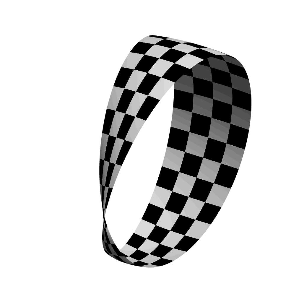
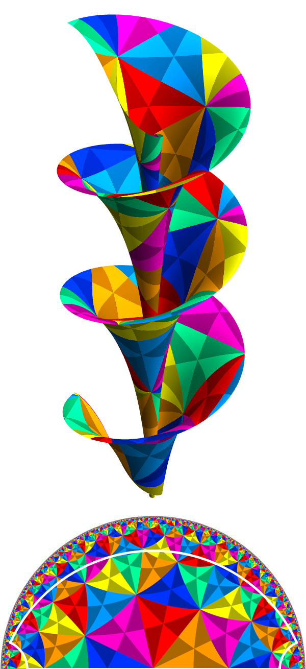
Escher’s “Circle Limit III” tiling shown on Dini’s surface: a surface built from helices with the same geometry as part of the hyperbolic plane.
|
|
Escher’s “Circle Limit III” tiling shown on Dini’s surface: a surface built from helices with the same geometry as part of the hyperbolic plane. |
A sheet of paper or a piece of fabric can lie perfectly flat on a table, but it can also be rolled up into a cylinder or a cone, and twisted in certain ways, without being stretched or sheared. Figures drawn on the material when it lies flat retain their shape, in the sense that distances measured within the material itself are unchanged by the way it happens to sit in three-dimensional space.
The geometry of ordinary paper is flat, Euclidean geometry, but what about the equivalent for spherical geometry (which would be something like a piece of orange peel), or for hyperbolic geometry?
The aim of this page is to investigate the possibilities for all three cases: given a piece of an idealised two-dimensional material whose geometry is Euclidean, spherical, or hyperbolic, what shapes can it adopt in three-dimensional Euclidean space?
There are three kinds of two-dimensional space that have constant Gaussian curvature, K:
[There are also spaces that consist of pieces of these spaces, with boundaries, or pieces where all or some of the boundaries have been joined together.]
Gaussian curvature, K, is a number that quantifies the manner and extent in which the geometry of a two-dimensional space departs from Euclidean geometry. It can be defined in many different ways, but one approach is to look at the geometry of a circle: the set of points that lie at a fixed distance from a given point, where we need to measure this along the geodesic curves that minimise the distance between points.
On the surface of a sphere with radius a, we measure distances along great circles, and a circle of radius r centred on the pole in spherical coordinates will lie at an angle of θ = r/a radians from the pole. A straightforward calculation gives the circumference and area of such a circle:
Circumference(r) = 2 π a sin(r/a)
Area(r) = 2 π a2 (1 – cos(r/a))
In general, a two-dimensional space might have different curvature at different points, but we can still characterise the local geometry by examining the limiting behaviour as the radius r of the circle becomes very small. If we take the first two non-zero terms of the Taylor series for the formulas above, we get:
Circumference(r) ≈ 2 π r – (π/(3 a2)) r3
Area(r) ≈ π r2 – (π/(12 a2)) r4
We can quantify the extent to which these formulas deviate from the usual Euclidean formulas for circumference and area, 2 π r and π r2, by defining the Gaussian curvature K to be either:
K = (3/π) limr → 0 (2 π r – Circumference(r)) / r3
or:
K = (12/π) limr → 0 (π r 2 – Area(r)) / r4
For the case of a sphere of radius a, both definitions yield:
K = 1 / a2
Another way of characterising Gaussian curvature is via the notion of angular excess. For any triangle in the plane whose sides are straight line segments, the sum of the three interior angles at the vertices is exactly π. On a sphere of radius a, the sum of the three angles for a triangle whose sides are geodesics depends on the area of the triangle, A. Specifically:
Sum-of-angles(A) = π + A/a2 = π + K A
We won’t prove this, but it is easy to check for some simple cases. For example, a triangle with one vertex at the north pole, and two that are 90 degrees apart on the equator, will have an area one-eighth that of the whole sphere, or 4πa2/8 = πa2/2, and since all three angles are right-angles, the sum of its angles will be 3π/2, in agreement with the formula. The local value of the curvature K can be obtained in the limiting case of a small triangle:
K = limA→0 (Sum-of-angles(A) – π) / A
We have used a sphere to demonstrate how geometry is affected by positive Gaussian curvature, but exactly the same mathematical relationships hold in surfaces with negative curvature. So when K < 0, the circumference and area of a circle are larger than those of a circle of the same radius in the plane, and the sum of the three angles of a triangle whose sides are geodesics will be less than π.
The description we are given of a two-dimensional space will usually come in either of two forms. We might be told how the space has been embedded as a surface in three-dimensional Euclidean space, like the sphere we have just described. Or we might be given a description of the surface’s intrinsic geometry, in terms of a metric.
The appendix to this web page explains how the Gaussian curvature is calculated in both these cases. For a more comprehensive treatment, there are many good textbooks, such as Lipschutz,[1] that give a detailed account of “the classical theory of surfaces,” which deals with the geometry of two-dimensional spaces via surfaces embedded in three-dimensional space.
There are four kinds of surfaces embedded in three-dimensional Euclidean space that are intrinsically flat, with a constant Gaussian curvature of zero:
Some of these categories can be seen as either special cases or limiting cases of others; for example, cylinders are like cones whose apex is moved infinitely far away.
That planes are flat is not just obvious, it’s the case where, if our measure of intrinsic curvature gave any other result than zero, we would throw it away and look for a new one. To check that we don’t need to do that, note that we can parameterise any plane with the formula:
x(u, v) = P + u a + v b
where P is a point on the plane and a and b are two fixed, linearly independent vectors that are parallel to the plane. All three second derivatives of x(u, v) with respect to the parameters are zero, so the second fundamental form, S, of the surface, defined in the appendix, will be zero everywhere, making its determinant zero, while the first fundamental form, g, will have a non-zero determinant because a and b are linearly independent. So the Gaussian curvature, K = det(S) / det(g), will be zero.
Given a curve c(s) that lies in a plane, the cylinder generated by c(s) is the surface traced out by all the lines perpendicular to the plane that pass through points on c(s). If the curve is closed, the cylinder will be finite in one direction, and if the curve is self-intersecting, the cylinder will be a self-intersecting surface, but if the curve is infinitely long and never intersects itself, the cylinder will be infinite in all directions, and will be an embedding of the entire Euclidean plane.
Suppose the parameter s for the curve is its arc length, and let p be a unit-length normal to the plane of the curve (we will reserve n for the normal vector to the cylinder itself). Then we can parameterise the cylinder as:
x(u, v) = c(u) + v p
Following the methods described in the appendix, we have:
xu = c'(u)
xv = p
n = xu × xv / |xu × xv| = c'(u) × p
xuu = c''(u)
xuv = 0
xvv = 0
g(u, v) =
xu · xu xu · xv xu · xv xv · xv =
1 0 0 1 S(u, v) =
xuu · n xuv · n xuv · n xvv · n =
c''(u) · n 0 0 0
K = det(S) / det(g) = 0 / 1 = 0
There is an easy way to construct an isometry (a one-to-one distance-preserving function) between these cylinders and all or part of the Euclidean plane: we map the point with coordinates (u, v) on the cylinder to the point (x, y) in the usual Cartesian coordinates on the plane, setting:
x = u
y = v
The metric in u, v coordinates is exactly the same as the Euclidean metric, so this map preserves distances and angles measured within the embedded surface.
If the curve c(s) never intersects itself, in the case of an infinitely long curve we get an isometry between the entire Euclidean plane and the cylinder. For finite curves, or if we choose to limit the range of the v coordinate, the isometry is with a piece of the plane.
If the cylinder is generated by a closed curve, the topology is no longer that of a piece of the plane, but that of a piece with two opposite edges joined together. Locally, the distinction is not important, and the Gaussian curvature remains zero everywhere, but obviously a circular cylinder is not globally isometric to a rectangle, or a strip of finite width, because some points on the opposite edges end up closer to each other in the cylinder.
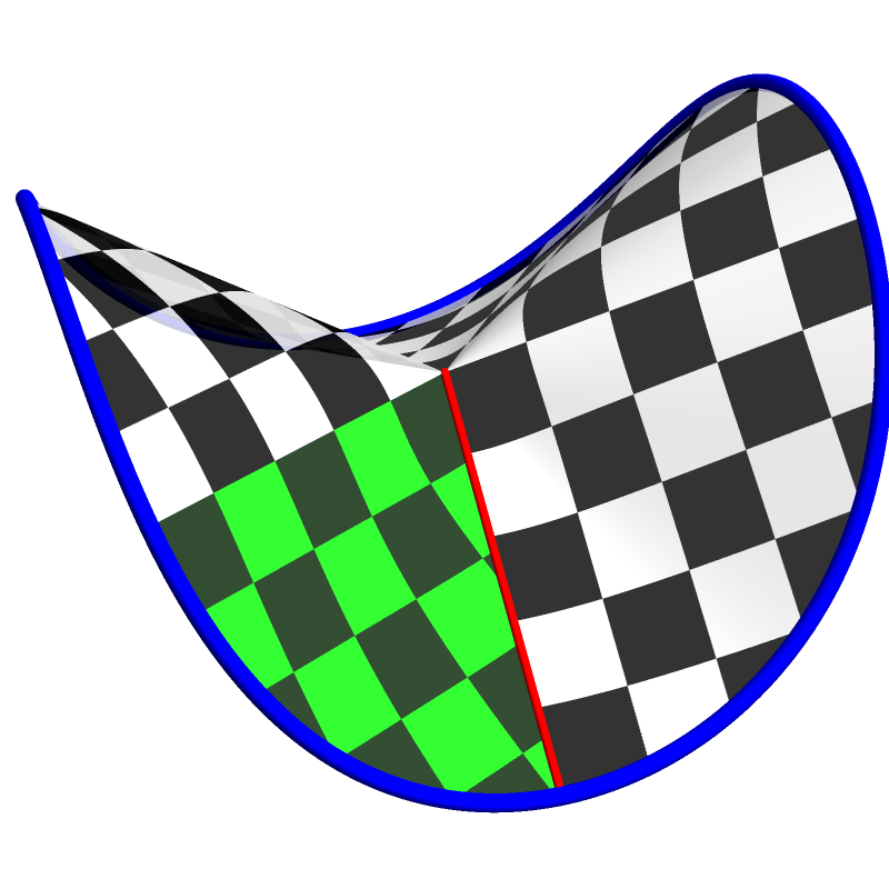
Green region comes from second copy of the plane
We will define a cone as the surface traced out by all the lines that pass through a curve c(s) and some fixed point A, the apex of the cone, which does not lie on the curve. Unlike the cylinder, we will not require c(s) to be planar, but we will impose the condition that the tangent to the curve never points directly towards the apex. We can parameterise this surface as:
x(u, v) = A + v (c(u) – A)
The original curve is given by v = 1, and the apex by v = 0. We then have, for v ≠ 0, and assuming c(s) is parameterised by arc length:
xu = v c'(u)
xv = c(u) – A
n = xu × xv / |xu × xv| = v c'(u) × (c(u) – A) / |v c'(u) × (c(u) – A)|
xuu = v c''(u)
xuv = c'(u)
xvv = 0
g(u, v) =
xu · xu xu · xv xu · xv xv · xv =
v2 v c'(u) · (c(u) – A) v c'(u) · (c(u) – A) |c(u) – A|2 S(u, v) =
xuu · n xuv · n xuv · n xvv · n =
v c''(u) · n 0 0 0
K = det(S) / det(g) = 0 / (v2 (|c(u) – A|2 – (c'(u) · (c(u) – A))2)) = 0
In general, the apex, v = 0, will not contain a neighbourhood that looks like part of a plane, so it needs to be excluded, and the surfaces with v < 0 and v > 0 are not connected to each other. Depending on the exact shape of the curve and the relative location of the apex, cones might or might not be self-intersecting elsewhere.
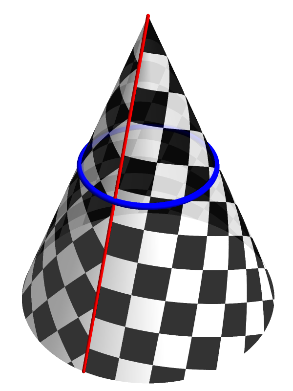
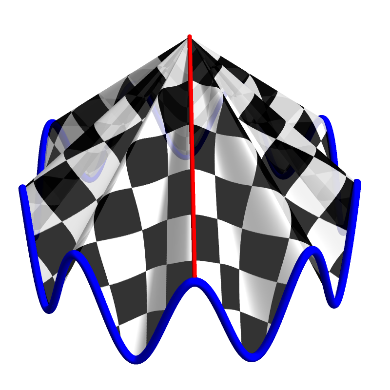
The most familiar example of a cone is a right circular cone, generated by a circle and an apex that lies directly above the centre of the circle. The portion of the plane that is embedded as a right circular cone is always a wedge with an angle less than 2π. However, cones generated by sufficiently meandering curves can come from wedges of any angle, including angles greater than or equal to 2π.
If the wedge angle is exactly 2π, as in the second illustration at the start of this section, then the cone might or might not count as an embedding of the entire Euclidean plane, depending on how strict we want to be about the smoothness of the embedding at the apex. If the wedge angle is greater than 2π, as in the third illustration, then the cone cannot be an embedding of just one copy of the Euclidean plane (in the illustration, an extra piece that comes from a second copy of the plane is coloured green). But it will still be a perfectly good intrinsically flat space, so long as we exclude the apex.
To construct an isometry between a cone described in the (u, v) coordinates we used in the definition, and part of the plane (or maybe parts of more than one plane), it is easiest if we work in polar coordinates (r, θ). An isometry is then given by:
r = v |c(u) – A|
θ = ∫0u (1/|c(t) – A|) √[1 – ((c(t) – A) · c'(t))2 / |c(t) – A|2] dt
The integral for θ amounts to adding up the distance we travel along the curve perpendicular to a line towards the apex, divided by the distance to the apex, to give us the angle we have travelled “around” the apex to reach the coordinate value u.
For example, if c(s) is a circle of radius R and the apex lies at a distance H directly above the centre of the circle, we have:
c(s) = (R cos(s/R), R sin(s/R), 0)
A = (0, 0, H)
|c(s) – A| = |(R cos(s/R), R sin(s/R), –H)| = √(R2 + H2)
r = v |c(u) – A| = v √(R2 + H2)
θ = ∫0u (1/|c(t) – A|) √[1 – ((c(t) – A) · c'(t))2 / |c(t) – A|2] dt
= (1/√(R2 + H2)) ∫0u √[1 – ((R cos(t/R), R sin(t/R), –H) · (–sin(t/R), cos(t/R), 0))2 / (R2 + H2)] dt
= u/√(R2 + H2)
The u coordinate will range from 0 to 2πR, so θ will range from 0 to 2πR/√(R2 + H2). This confirms that any right circular cone has a wedge angle of less than 2π. But for other cones, if θ exceeds 2π we will need to obtain the remainder of the surface from one or more extra copies of the plane.
with v > 0 in yellow,
v < 0 in red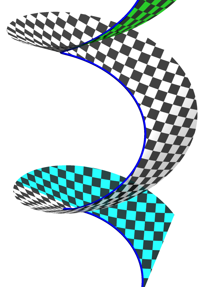
to diffferent copies of the plane
Suppose we have a curve c(s), parameterised by arc length s, that has no points of inflection: that is, no points where the unit-length tangent to the curve, c'(s), has a rate of change of zero as we move along the curve. This is the same as saying that for all s, c''(s) ≠ 0.
The tangent surface of c(s) is the surface consisting of all lines that are tangents to the curve. [In some literature, this is called the tangent developable; the term “developable” refers to any intrinsically flat surface.] We can parameterise the tangent surface as:
x(u, v) = c(u) + v c'(u)
Because c(s) is parameterised by arc length, c'(s) has a constant length of 1, and its rate of change, c''(s), is always orthogonal to it, since it can only change direction, not length. We then have, for v ≠ 0:
xu = c'(u) + v c''(u)
xv = c'(u)
n = xu × xv / |xu × xv| = v c''(u) × c'(u) / |v c''(u) × c'(u)|
xuu = c''(u) + v c'''(u)
xuv = c''(u)
xvv = 0
g(u, v) =
xu · xu xu · xv xu · xv xv · xv =
1 + v2 |c''(u)|2 1 1 1 S(u, v) =
xuu · n xuv · n xuv · n xvv · n =
v c'''(u) · n 0 0 0
K = det(S) / det(g) = 0 / (v2 |c''(u)|2) = 0
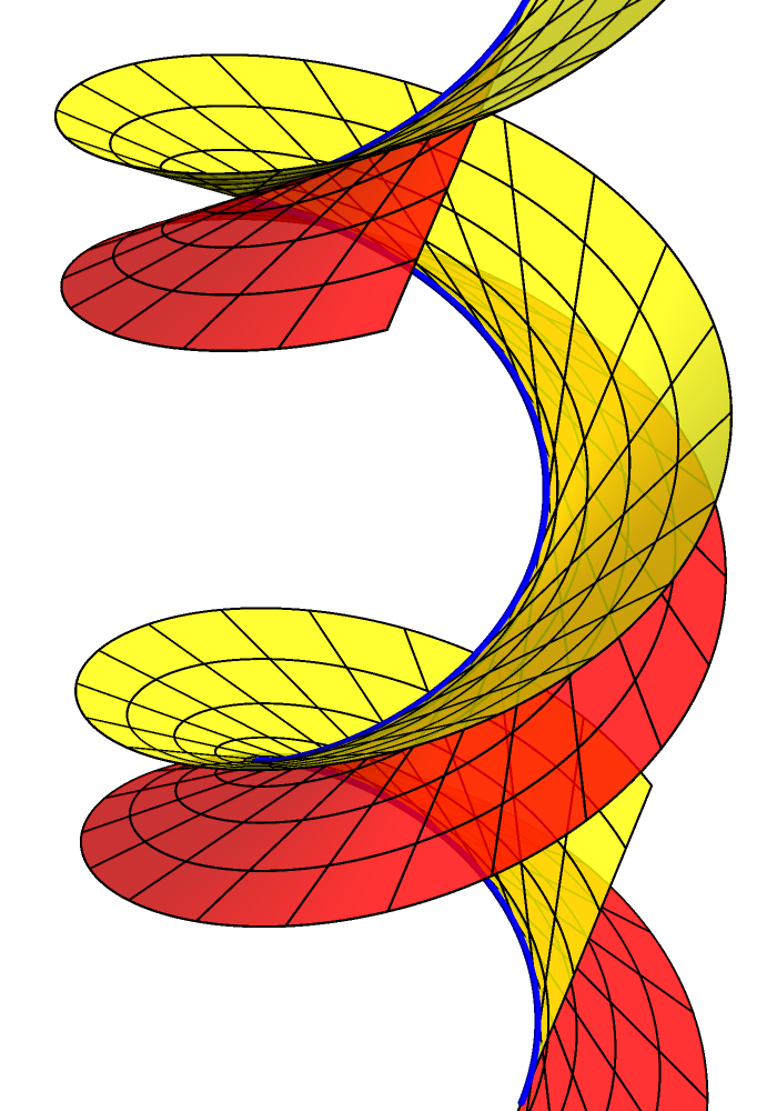
It might not be immediately obvious from our definitions, but we do not obtain a single, smooth surface if we allow the v coordinate to take on both positive and negative values. The first figure at the start of this section makes this clear; the yellow and red surfaces meet along the generating curve, but there is a cusp where they come together, rather than a smooth transition.
To find an isometry between a tangent surface and part of the plane, we will focus on the particular example of the tangent surface to a helix, h(s), with radius a and pitch controlled by b:
We define a parameter c = √(a2 + b2)
h(s) = (a cos(s/c), a sin(s/c), b s/c)
h'(s) = (–a/c sin(s/c), a/c cos(s/c), b/c)
h''(s) = (–a/c2 cos(s/c), –a/c2 sin(s/c), 0)
h'''(s) = (a/c3 sin(s/c), –a/c3 cos(s/c), 0)
x(u, v) = h(u) + v h'(u) = (a cos(u/c), a sin(u/c), b u/c) + v (–a/c sin(u/c), a/c cos(u/c), b/c)
xu = h'(u) + v h''(u) = (–a/c sin(u/c), a/c cos(u/c), b/c) + v (–a/c2 cos(u/c), –a/c2 sin(u/c), 0)
xv = h'(u) = (–a/c sin(u/c), a/c cos(u/c), b/c)
n = v h''(u) × h'(u) / |v h''(u) × h'(u)| = sign(v) (–b/c sin(u/c), b/c cos(u/c), –a/c)
xuu = h''(u) + v h'''(u) = (–a/c2 cos(u/c), –a/c2 sin(u/c), 0) + v (a/c3 sin(u/c), –a/c3 cos(u/c), 0)
xuv = h''(u) = (–a/c2 cos(u/c), –a/c2 sin(u/c), 0)
xvv = 0
g(u, v) =
1 + v2 |h''(u)|2 1 1 1 =
1 + a2 v2 / c4 1 1 1 S(u, v) =
v h'''(u) · n 0 0 0 =
–sign(v) a b v / c4 0 0 0
To construct an isometry, we will first identify a convenient set of geodesics on the tangent surface, which will need to correspond to straight lines in the plane. To start, we will note that any straight line (in the sense of being straight in three-dimensional Euclidean space) in any smoothly embedded surface is a geodesic.[4] So the lines of fixed u and varying v in a tangent surface are all geodesics.
To find other geodesics, we will make use of the fact that the metric for the helix tangent surface is completely independent of the u coordinate. It follows that changing u by a fixed amount everywhere maps the surface into itself isometrically; that is, it is a symmetry of the surface, which corresponds to a screwlike motion, where we rotate the surface around the axis of the helix while also moving everything along the axis.
A further consequence of this is that, along any geodesic G(s), the dot product between the tangent to the geodesic, G'(s), and the vector field that corresponds to a uniform change in the u coordinate, which is just (1,0) in (u, v) coordinates, is constant. This result is known as Killing’s theorem, and it is described in a bit more detail here [this article is associated with my novel Incandescence, but there is no need to know anything about that book to follow the discussion of the geometry].
So, Killing’s theorem gives us, for a geodesic:
G(s) = (uG(s), vG(s))
with tangent vector:
G'(s) = (uG'(s), vG'(s))
a conserved quantity C along the geodesic:
G'(s)T g(G(s)) (1,0) = C
(1 + a2 vG(s)2 / c4) uG'(s) + vG'(s) = C
We can check this for the geodesics we already know about, the lines of constant u and varying v:
uG(s) = u0
vG(s) = s
uG'(s) = 0
vG'(s) = 1
(1 + a2 vG(s)2 / c4) uG'(s) + vG'(s) = 1
If the geodesic is parameterised by arc length, its tangent will have a length of 1 everywhere, and we can use that to solve for uG'(s) in terms of vG(s) and vG'(s).
G'(s)T g(G(s)) G'(s) = 1
(1 + a2 vG(s)2 / c4) uG'(s)2 + 2 uG'(s) vG'(s) + vG'(s)2 = 1
uG'(s) = (–vG'(s) ± √[1 + (a2/c4) vG(s)2 (1 – vG'(s)2)]) / (1 + a2 vG(s)2 / c4)
With this result, we have for the conserved quantity along the geodesic:
(1 + a2 vG(s)2 / c4) uG'(s) + vG'(s) = C
± √[1 + (a2/c4) vG(s)2 (1 – vG'(s)2)] = C
1 + (a2/c4) vG(s)2 (1 – vG'(s)2) = C2
Suppose we want to find a geodesic that meets one of our straight-line geodesics of constant u at some point (u0, v0), and the two geodesics are orthogonal to each other where they meet, at s = 0. Then we will want the tangent to the geodesic at s = 0 to be:
G'(0) = (uG'(0), vG'(0)) = (c2 / (a v0), –c2 / (a v0))
since this tangent has unit length, and it is orthogonal to (0,1), the tangent to the straight-line geodesic:
G'(0)T g(u0, v0) G'(0) = 1
G'(0)T g(u0, v0) (0,1) = 0
The initial value this gives us for vG'(0) lets us compute the conserved quantity at the start of the geodesic:
C2 = 1 + (a2/c4) vG(s)2 (1 – vG'(s)2) = (a2/c4) v02
and the differential equation we need to solve becomes:
1 + (a2/c4) vG(s)2 (1 – vG'(s)2) = (a2/c4) v02
with the initial conditions:
vG(0) = v0
vG'(0) = –c2 / (a v0)
This is solved by:
vG(s) = √[s2 – 2 (c2/a) s + v02]
If we look at the points in the (s, v0) plane where vG(s) = 0, it turns out they lie on a circle, with radius c2/a, and centre (c2/a, 0). This circle in the (s, v0) plane corresponds to the helix in the tangent surface, and vG(s) is precisely the distance from (s, v0) to this circle, measured along a tangent to the circle.
A line of constant v0 in the (s, v0) plane with |v0| < c2/a will intersect the circle, and for values of s that lie inside the circle, vG(s) becomes imaginary. In other words, these geodesics of constant v0 reach the boundary of the tangent surface, the helix, and come to an end there. But for |v0| > c2/a these geodesics never hit the boundary. Similarly, geodesics of constant s and varying v0 will only hit the boundary and come to an end if 0 < s < 2c2/a.
If we substitute this solution for vG(s) back into our original equation for the conserved quantity, before we eliminated uG'(s), we can now solve that equation for uG'(s) and integrate it to find uG(s). The solution we obtain is:
uG(s) = u0 + 2 (c2/a) arctan(s / (v0 + vG(s)))
How does uG(s) relate to the circle in the (s, v0) plane that corresponds to the helix? For points that lie on that circle, it must equal u0 plus the arc length along the circle, measured from the origin. This means that throughout the (s, v0) plane, the range of u values is limited to the interval u0 ± π (c2/a), and a single copy of the plane can only correspond to that portion of the tangent surface.
So the isometry we have found maps regions of the helix tangent surface where the u coordinate changes by 2π (c2/a) to copies of the plane with a disk of radius c2/a cut out of it. The second figure at the start of this section uses different colours to show the different copies of the plane that are mapped to the surface.
Note that the curvature of the generating helix, as a curve in three-dimensional Euclidean space:
κ = |h''(s)| = a/c2
is precisely the curvature (the inverse of the radius, c2/a) of the corresponding circle in the plane. This is certainly not true in general for the images of curves under this isometry; for example, most straight lines in the plane do not map to straight lines in three-dimensional space. However, it is not a coincidence either; the generating curve of any tangent surface always has the same curvature in three-dimensional Euclidean space as it has intrinsically as a curve in the tangent surface, or equivalently, as the corresponding curve under an isometry with the Euclidean plane.
that is not intrinsically flat.
All four kinds of intrinsically flat surfaces we have described are examples of ruled surfaces: surfaces that are built entirely from a family of straight lines. But not every ruled surface is intrinsically flat. If we compute the Gaussian curvature of an arbitrary ruled surface, what further conditions are required to ensure that K = 0?
Suppose we have a curve, c(s), parameterised by arc length, and at each point on the curve there is a unit-length vector L(s) that gives the direction of the straight line passing through that point. The resulting surface is parameterised as:
x(u, v) = c(u) + v L(u)
We perform the usual calculations to find the Gaussian curvature:
xu = c'(u) + v L'(u)
xv = L(u)
n = xu × xv / |xu × xv| = (c'(u) + v L'(u)) × L(u) / |(c'(u) + v L'(u)) × L(u)|
= (c'(u) + v L'(u)) × L(u) / √(|c'(u) + v L'(u)|2 – (c'(u) · L(u))2)
xuu = c''(u) + v L''(u)
xuv = L'(u)
xvv = 0
g(u, v) =
xu · xu xu · xv xu · xv xv · xv =
|c'(u) + v L'(u)|2 c'(u) · L(u) c'(u) · L(u) 1 S(u, v) =
xuu · n xuv · n xuv · n xvv · n =
(c''(u) + v L''(u)) · n L'(u) · n L'(u) · n 0
K = det(S) / det(g) = –[L'(u) · c'(u) × L(u) / (|c'(u) + v L'(u)|2 – (c'(u) · L(u))2)]2
This expression for the curvature tells us that it can never be positive, since it is the opposite of a squared real-valued quantity. What’s more, it cannot be equal to a constant negative value, since the only way to remove the dependence on v would involve either setting L'(u) = 0, or otherwise making the numerator zero, both of which would produce flat surfaces.
But the ruled surface will be intrinsically flat if, and only if:
L'(u) · c'(u) × L(u) = 0
This scalar triple product will obviously be zero if one or more of the three vectors are zero. But it will also be zero if any two of the vectors are parallel, or if all three vectors are coplanar.
Are there are any other possibilities besides these four cases? We can splice different kinds of surface together, e.g. we could join a cone and a cylinder, but locally, is there any other way to meet this condition on the ruled surface that we haven’t already considered?
The answer is no; this list is complete! Here is a proof, taken from Lipschutz.[5]
The condition that the scalar triple product L'(u) · c'(u) × L(u) = 0 means there must be three functions, α(u), β(u), γ(u), which demonstrate the linear dependence of the three vectors:
α(u) c'(u) + β(u) L(u) + γ(u) L'(u) = 0
α(u), β(u), γ(u) are never all equal to zero for the same value of u.
This must be true for the entire range of the u parameter relevant to the surface in question, but it’s possible that different subsets of {α(u), β(u), γ(u)} will be zero on various intervals of the parameter.
Case 1. Suppose α(u) = 0 on some interval for u. Then on that interval, the original condition becomes:
β(u) L(u) + γ(u) L'(u) = 0
β(u), γ(u) are never both equal to zero for the same value of u.
Because L(u) is a unit vector, its derivative is always orthogonal to it, and we have:
L(u) · (β(u) L(u) + γ(u) L'(u)) = β(u) = 0
γ(u) L'(u) = 0, and γ(u) ≠ 0 because β(u) = 0
So L'(u) = 0
This means L(u) is a constant vector, and the portion of the surface corresponding to this interval must be a generalised cylinder (which includes the plane as a special case).
Case 2. Suppose α(u) ≠ 0 on some interval for u. Then we can solve the original equation for c'(u):
c'(u) = –β(u)/α(u) L(u) – γ(u)/α(u) L'(u)
We will define a new curve, C(u), as:
C(u) = c(u) + γ(u)/α(u) L(u)
Differentiating with respect to u, we have:
C'(u) = c'(u) + d(γ(u)/α(u))/du L(u) + γ(u)/α(u) L'(u)
= η(u) L(u)
where we have defined η(u) as:
η(u) = d(γ(u)/α(u))/du – β(u)/α(u)
Case 2A. Suppose η(u) = 0 on some sub-interval of the one we are considering where α(u) ≠ 0. Then on that sub-interval we have:
C'(u) = 0
C(u) = A, for some constant vector A
c(u) = A – γ(u)/α(u) L(u)
x(u, v) = A + (v – γ(u)/α(u)) L(u)
This means that all the lines that generate the surface pass through A, and the surface must either be a generalised cone with apex A, or part of a plane.
Case 2B. Suppose η(u) ≠ 0 on some sub-interval. Then we have:
L(u) = C'(u) / η(u)
c(u) = C(u) – γ(u)/α(u) L(u) = C(u) – γ(u)/[α(u) η(u)] C'(u)
x(u, v) = c(u) + v L(u) = C(u) + (v/η(u) – γ(u)/[α(u) η(u)]) C'(u)
This means the lines that generate the surface are all tangents to the curve C(u), and the surface here is part of the tangent surface to C(u).
The one remaining question is whether there is any way to have an intrinsically flat surface that is not a ruled surface. The answer to that is no;[6] we won’t reproduce the proof here, but it formalises the intuitive idea that if, at every point, one of the principal curvatures of the surface is zero, then if you keep moving across the surface in the corresponding direction, you must be following a straight line in three-dimensional space.
Given a smooth, non-self-intersecting curve c(s) in three-dimensional Euclidean space, is it possible to find an intrinsically flat surface in which that curve is a geodesic? Intuition suggests that the answer should be yes: a strip of (perfectly flexible) paper, narrow enough that it won’t bump into itself in any tight places on the curve, could be positioned so that its centreline coincides with the curve.
The surface that meets this condition is known as the rectifying developable for the curve.[7] We know from the previous section that it will be a ruled surface, so we can parameterise it as:
x(u, v) = c(u) + v L(u)
for some L(u) yet to be determined, which we will write initially as:
L(u) = A(u) c'(u) + B(u) c''(u) + D(u) c'(u) × c''(u)
A normal vector to the surface at any point on the curve c(u) will be given by:
N(u) = L(u) × c'(u)
= B(u) c''(u) × c'(u) + D(u) (c'(u) × c''(u)) × c'(u)
= B(u) c''(u) × c'(u) + D(u) c''(u)
Along a geodesic, the tangent to the curve, c'(u), its derivative, c''(u), and the normal vector to the surface, N(u), all lie in the same plane.[3] So to make c(u) a geodesic, we must have:
N(u) · (c'(u) × c''(u)) = 0
which requires (assuming c''(u) is nonzero) that B(u) = 0. Then the condition for this ruled surface to be intrinsically flat is:
L'(u) · c'(u) × L(u) = 0
[A'(u) c'(u) + A(u) c''(u) + D'(u) c'(u) × c''(u) + D(u) c'(u) × c'''(u)] · [c'(u) × (A(u) c'(u) + D(u) c'(u) × c''(u))] = 0
[A'(u) c'(u) + A(u) c''(u) + D'(u) c'(u) × c''(u) + D(u) c'(u) × c'''(u)] · [–D(u) c''(u)] = 0
A(u) |c''(u)|2 + D(u) (c'(u) × c'''(u)) · c''(u) = 0
A(u) κ2(u) – D(u) κ2(u) τ(u) = 0
Here κ(u) is the length of c''(u), which measures the curvature of c(u), and τ(u) is the torsion of the curve, which measures the rate at which the plane of the curve is changing its orientation as we move along the curve. There are several different formulas that all yield this quantity, but for our purposes the most convenient formula is:
τ(s) = (c'(s) × c''(s)) · c'''(s) / κ(s)2
If we want L(u) to be a unit-length vector, this condition will be satisfied by:
L(u) = (τ(u) c'(u) + c'(u) × c''(u)) / √[τ(u)2 + κ(u)2]
The numerator here is a vector associated with the curve, known as the Darboux vector, which describes the “angular velocity” of the orthogonal set of axes given by the unit-length tangent to the curve, c'(u), its derivative, c''(u), and their cross product, as we move along the curve. (It is common practice to also normalise the last two vectors to unit length, giving an orthonormal frame known as the Frenet-Serret frame.)
So, if we take a smooth, non-self-intersecting curve and construct a ruled surface whose lines lie in the direction of the Darboux vector at each point on the curve, the curve will be a geodesic for that surface.
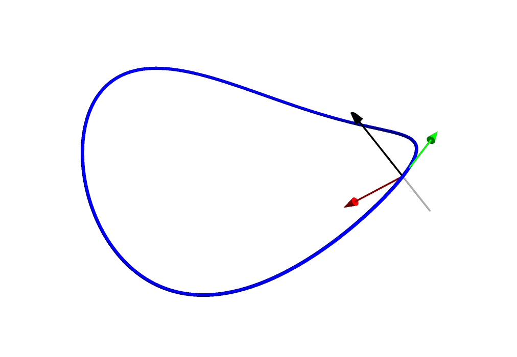
The Frenet-Serret frame for the blue curve
(green tangent, red normal, black binormal)
with the Darboux vector providing the rulings (grey)
for an intrinsically flat surface.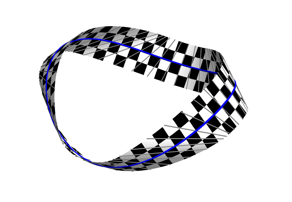
These surfaces are the rectifying developables for the blue curves,
with the
Darboux vector rulings shown in grey.
If c(u) is a straight line, the Darboux vector will be undefined, but we can use any plane that contains that line as a surface with the required properties.
The next simplest case would be a planar curve. This will have zero torsion, so L(u) will be a fixed vector perpendicular to the plane of the curve, giving us a cylinder. Similarly, if we choose a curve that is a geodesic on a cone, the rectifying developable will be that cone.
But generically, the surface we get from a curve will be a tangent surface, and we can explicitly identify the curve whose tangents are the same set of straight lines as we get from the Darboux vectors of the original curve. If we define:
T(s) = c(s) + [κ(s)/(τ(s) κ'(s) – τ'(s) κ(s))] (τ(s) c'(s) + c'(s) × c''(s))
then it turns out that T'(s) is parallel to the Darboux vector for c(s), so the tangent surface for T(s) is the rectifying developable for c(s). Note that the parameter s here is an arc length parameter for c(s) only, and not for T(s).
T(s) will constitute an edge to the surface, just as any curve does for its own tangent surface. The distance measured along the ruling line from the point c(s) to the edge of the surface will be:
Distance to edge along ruling
= | κ(s) √[τ(s)2 + κ(s)2] / (τ(s) κ'(s) – τ'(s) κ(s)) |
If we want to know the orthogonal distance, measured within the surface, between a point on the edge, T(s), and the generating curve (which is a geodesic for the surface), we can make use of the fact that the sine of the angle between the ruling lines and the curve is κ(s)/√[τ(s)2 + κ(s)2], from which we obtain:
Orthogonal distance from edge to prescribed geodesic
= | κ(s)2 / (τ(s) κ'(s) – τ'(s) κ(s)) |
= | 1 / d(τ(s)/κ(s))/ds |
We can also use that formula for the the sine of the angle between the ruling lines and the curve to write an isometry between the rectifying developable and the plane, in Cartesian coordinates (x, y):
x = u + v (τ(u)/√[τ(u)2 + κ(u)2])
y = v (κ(u)/√[τ(u)2 + κ(u)2])
If the curvature vector c''(u) is zero at an isolated point u0, the unit-length normal vector c''(u)/|c''(u)|, which is undefined at u0, can either have the same, or opposite, limiting values on either side of u0. If the torsion also goes to zero at the same point, the normalised Darboux vector we are using for L(u) can also switch direction. This doesn’t affect the surface itself (since the ruling lines, which follow the Darboux vector in both directions, are unchanged) but in order to make the (u, v) coordinates continuous across the change, we can multiply L(u) by a sign that is chosen in order to extend continuity as much as possible.
If the torsion does not go to zero at a point where the curvature does, then that marks a point where c(s) intersects the edge curve T(s).
If we construct the rectifying developable for a smooth closed curve on which the curvature is never zero, then the surface will be topologically a cylinder: a piece of the plane whose opposite edges join up without a twist. But if there are an odd number of points of zero curvature and torsion where the direction of the normalised curvature and Darboux vectors change discontinuously, the surface will be a Möbius strip.
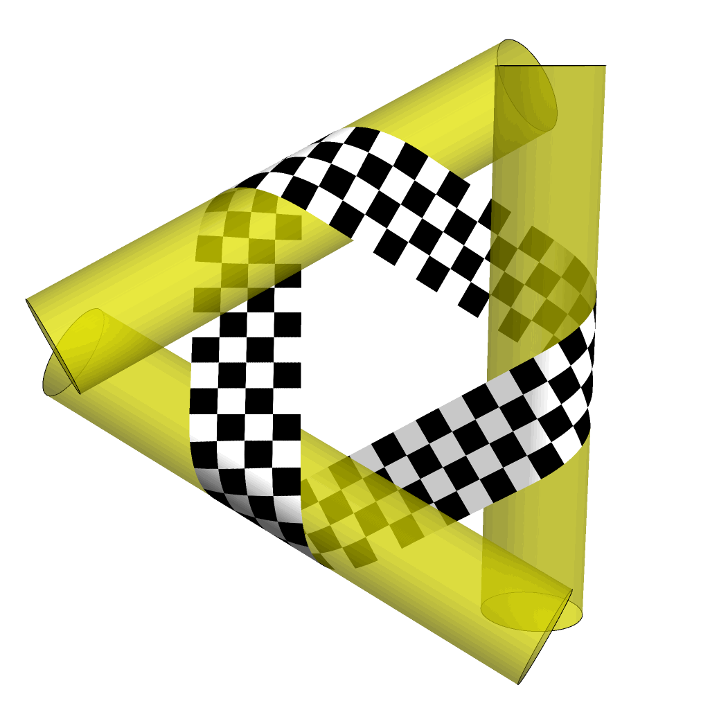
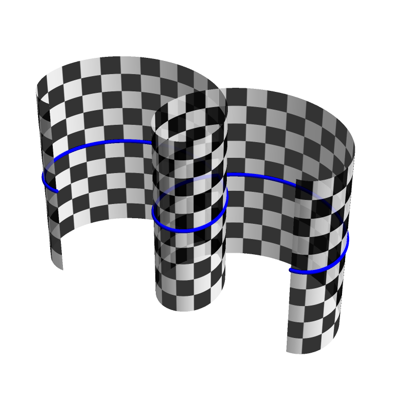
A Möbius strip whose centreline is
a piecewise curve of helices and line segments.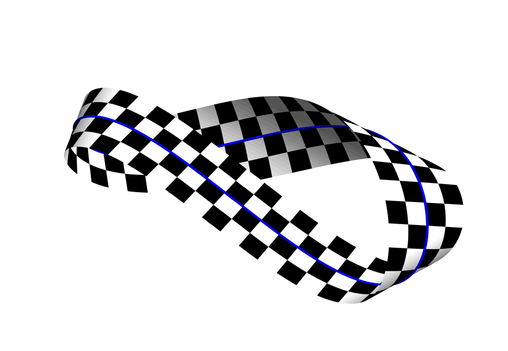
A Möbius strip whose centreline is
the smooth curve
(3 sin(t), cos(t) + (2/5) cos(2t) + (1/15) cos(3t), (3/4) sin(2t)).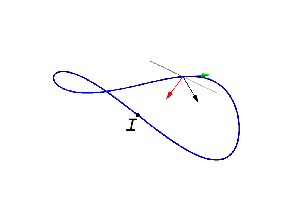
The Frenet-Serret frame for the blue curve
(green tangent, red normal, black binormal)
with the Darboux vector providing the rulings (grey)
for the Möbius strip.
We can embed a Möbius strip isometrically in three dimensions by wrapping the strip around three cylinders, as in the first image above. In this case, the centreline is a piecewise function that splices together three helices and three line segments, and the surface is spliced together from three cylindrical regions and three planar regions.
We can also embed a Möbius strip as the rectifying developable of a single smooth curve, as in the second image above. The third image shows what is happening with the Frenet-Serret frame. The red vector would change direction at the inflection point, I, if we simply defined it as c''(u)/|c''(u)|, but we multiply it with a sign that makes it continuous as it crosses that point. However, as a result of that single change of sign, it no longer agrees with its original direction when it comes full circle; it needs to traverse the loop twice before that happens. This is accompanied by a similar change in the Darboux vector, so the ruling lines reverse orientation after a single circuit around the loop, making the surface a Möbius strip.
The function we have chosen for the y coordinate of the curve might look a bit strange and arbitrary at first glance:
y(t) = cos(t) + (2/5) cos(2t) + (1/15) cos(3t)
In fact, this is the simplest trigonometric function with a Taylor series at π that is a constant plus a sixth-order term:
y(π + ε) ≈ –2/3 + (1/30) ε6
This produces an inflection point at π with suitable behaviour for the curvature and torsion: both go to zero, but the torsion must go to zero at least as rapidly as the curvature, in order for the width of the strip we can fit around the centreline, |1 / d(τ(s)/κ(s))/ds|, to remain non-zero. Because we have chosen to make the curve symmetrical under a 180° rotation around the y-axis, the torsion must be an even function of ε, so the lowest order it can have is quadratic.
κ(π + ε) ≈ (4/(5√5)) |ε|
τ(π + ε) ≈ –(2/9) ε2
A sequence of projections of a single Möbius strip
in four-dimensional space down to three dimensions.
Although this web page is focused on surfaces embedded in three-dimensional space, we will note that embeddings in four dimensions allow for more possibilities. Intrinsically flat surfaces in four dimensions need not be ruled surfaces, and some topologies that cannot be embedded in three dimensions because the surface will unavoidably intersect itself can be embedded in four dimensions.
Consider the following surface embedded in four dimensions, parameterised as:
x(u, v) = (cos u cos v, sin u cos v, 2 cos(u/2) sin v, 2 sin(u/2) sin v)
In four dimensions, we can still use the methods described in the appendix to find the metric:
xu = (–sin u cos v, cos u cos v, –sin(u/2) sin v, cos(u/2) sin v)
xv = (–cos u sin v, –sin u sin v, 2 cos(u/2) cos v, 2 sin(u/2) cos v)
g(u, v) =
xu · xu xu · xv xu · xv xv · xv =
1 0 0 1+3 cos2 v
While we could proceed to compute the Gaussian curvature from the metric with the whole apparatus of Christoffel symbols and the Riemann curvature tensor described in the second appendix, we don’t actually need to do all that work to conclude that the surface is intrinsically flat! The metric is already almost in the form of the two-dimensional Euclidean metric, except for the g22 component, which is a function of the second parameter v, rather than being 1.
But if we changed to a new parameter in place of v that measured arc length along each curve of varying v and constant u, then g22 would become 1, and the metric would be precisely the Euclidean metric, since this change would have no effect on the other components.
What is the topology of this surface? If we allow u to range from 0 to 2π, and v to range from –V to V for some value of V greater than 0 and strictly less than π, then we can examine how the two ends, u = 0 and u = 2π, of the coordinate rectangle are related in the embedding:
x(0, v) = (cos v, 0, 2 sin v, 0)
x(2π, v) = (cos v, 0, –2 sin v, 0)
x(2π, –v) = (cos v, 0, 2 sin v, 0)
We see that the two ends coincide, but with the value of the v coordinate negated, which amounts to a 180° twist. This is precisely the topology of a Möbius strip.
What if we set V = π, widening the strip so that v ranges from –π to π? We then have the other two sides of the coordinate rectangle meeting:
x(u, –π) = (–cos u, –sin u, 0, 0)
x(u, π) = (–cos u, –sin u, 0, 0)
Since these sides meet up with no change in orientation, this shows that the surface has closed up into a Klein’s bottle. Of course, it remains intrinsically flat, and there are no self-intersections (other than the required meeting of the borders of the coordinate rectangle). The “tube” of the Klein’s bottle is generated by taking an ellipse, given by the curve for varying v at u = 0:
x(0, v) = (cos v, 0, 2 sin v, 0)
and applying a continuous family of four-dimensional rotations to it, by an angle of u in the xy plane and an angle of u/2 in the zw plane, where we are calling the four coordinates (x, y, z, w).
The animation at the start of this section shows a single, rigid Möbius strip with this embedding, but it is projected down to three dimensions using the basis:
{(0, 0, cos α, sin α), (1, 0, 0, 0), (0, 1, 0, 0)}
with α cyling from 0 to 2π over the course of the animation. To be clear, these projections to three-dimensional space are not intrinsically flat.
We will start our exploration of surfaces of constant non-zero Gaussian curvature by looking for examples that can be produced by taking a planar curve and rotating it around an axis. This will certainly not encompass all the surfaces we want to catalogue, eventually, but the advantage of starting here is to find some examples while keeping the mathematics relatively simple, as these surfaces of revolution can be described with a single function of one variable.
One way to parameterise a surface of revolution is to describe the z coordinate as a function of the radial cylindrical coordinate, ρ, i.e. the distance from the axis. While we could reverse this, and describe the radius as a function of z, or, to allow for completely general curves, describe both ρ and z as functions of some parameter, the approach we have chosen will make our calculations easier, and the results simpler to express.
So, we will parameterise our surface as:
x(φ, ρ) = (ρ cos φ, ρ sin φ, f(ρ))
where the right-hand side here are ordinary Cartesian coordinates, x, y, z. We have departed from our earlier practice of using (u, v) as the names for the two surface coordinates, in favour of (φ, ρ), which are more suggestive of the geometry, at least for readers who have been exposed to the conventional choice of symbols for cylindrical coordinate systems.
Following the usual recipe for computing the Gaussian curvature of an embedded surface (spelled out in the appendix), we have:
xφ = (–ρ sin φ, ρ cos φ, 0)
xρ = (cos φ, sin φ, f '(ρ))
n = xφ × xρ / |xφ × xρ| = (f '(ρ) cos φ, f '(ρ) sin φ, –1) / √[1 + f '(ρ)2]
xφφ = (–ρ cos φ, –ρ sin φ, 0)
xφρ = (–sin φ, cos φ, 0)
xρρ = (0, 0, f ''(ρ))
g(φ, ρ) =
xφ · xφ xφ · xρ xφ · xρ xρ · xρ =
ρ2 0 0 1 + f '(ρ)2 S(φ, ρ) =
xφφ · n xφρ · n xφρ · n xρρ · n =
–ρ f '(ρ) / √[1 + f '(ρ)2] 0 0 –f ''(ρ) / √[1 + f '(ρ)2]
K = det(S) / det(g) = f '(ρ) f ''(ρ) / [ρ (1 + f '(ρ)2)2)]
To produce a surface of constant Gaussian curvature, K, we need to solve the differential equation here for f(ρ). As a first step, we can rewrite this as:
–1/(2 ρ) d(1/(1 + f '(ρ)2))/dρ = K
This is straightfoward to solve for f '(ρ):
d(1/(1 + f '(ρ)2))/dρ = –2 K ρ
1/(1 + f '(ρ)2) = –K ρ2 + c
f '(ρ) = ±√[1/(–K ρ2 + c) – 1]
Here c is a constant of integration. The values that c can take such that the quantity inside the square root remains non-negative for some non-empty range of values for ρ will depend on the sign of K. The condition we need to satisfy is:
0 < –K ρ2 + c < 1
That is to say, a parabola centred on ρ = 0 that either points down (if K > 0) or up (if K < 0), and which has a maximum or minimum value of c at ρ = 0, must lie between 0 and 1 for some non-empty range of values for ρ.
Suppose K = 1/a2, i.e. the Gaussian curvature takes the positive value that corresponds to a sphere of radius a. Then c must be greater than zero, or the downwards-pointing parabola will never take on any positive values. It will be convenient to set c = χ2. The range of values for ρ will then be:
| If 0 < χ ≤ 1 | 0 < ρ < a χ | |
| If χ > 1 | a √[χ2 – 1] < ρ < a χ |
Here f '(ρ) → ∞ as ρ → a χ, and f '(ρ) = 0 at ρ = a √[χ2 – 1].
For negative curvature, say K = –1/a2, we must have c less than 1, or the upwards-pointing parabola will never take on any values less than 1. In this case, we will set c = 1 – ξ2, and the range of values for ρ will be:
| If 0 < ξ ≤ 1 | 0 < ρ < a ξ | |
| If ξ > 1 | a √[ξ2 – 1] < ρ < a ξ |
We now have f '(ρ) → ∞ as ρ → a √[ξ2 – 1], and f '(ρ) = 0 at ρ = a ξ.
We can integrate our result for f '(ρ) to find f(ρ). For the special case c = 1, which is only compatible with positive curvature, so we will set K = 1/a2:
Sphere
K = 1/a2 c = 1
f '(ρ) = ±ρ / √[a2 – ρ2]
f(ρ) = zeq ∓ √[a2 – ρ2]
This is just the formula for two quadrants of a circle of radius a, and the resulting surface of revolution is a sphere of radius a, with the z coordinate of its equator given by the constant of integration zeq.
For the special case c = 0, which is only compatible with negative curvature:
Tractroid
K = –1/a2 c = 0
f '(ρ) = ±√[a2 – ρ2] / ρ
f(ρ) = zeq ± (√[a2 – ρ2] – a arccosh(a/ρ))
This function is called a tractrix, and its surface of revolution, a tractroid, is the most famous example of a pseudosphere: a surface of constant negative curvature.
If c ≠ 1 and c ≠ 0, we have:
Generic surface of revolution of constant Gaussian curvature K
f(ρ) = zeq ± √[(1 – c)/K] (E(arcsin(√[K/c] ρ) | c/(c – 1)) – e0)
If K > 0 e0 = E(c/(c – 1)) If K < 0 e0 = E(arcsin(√[(c – 1)/c]) | c/(c – 1))
The function E is an elliptic integral of the second kind, defined as:
E(s | m) = ∫0s √[1 – m sin2 t] dt = ∫0sin s √[1 – m u2] / √[1 – u2] du
E(m) = E(½π | m)
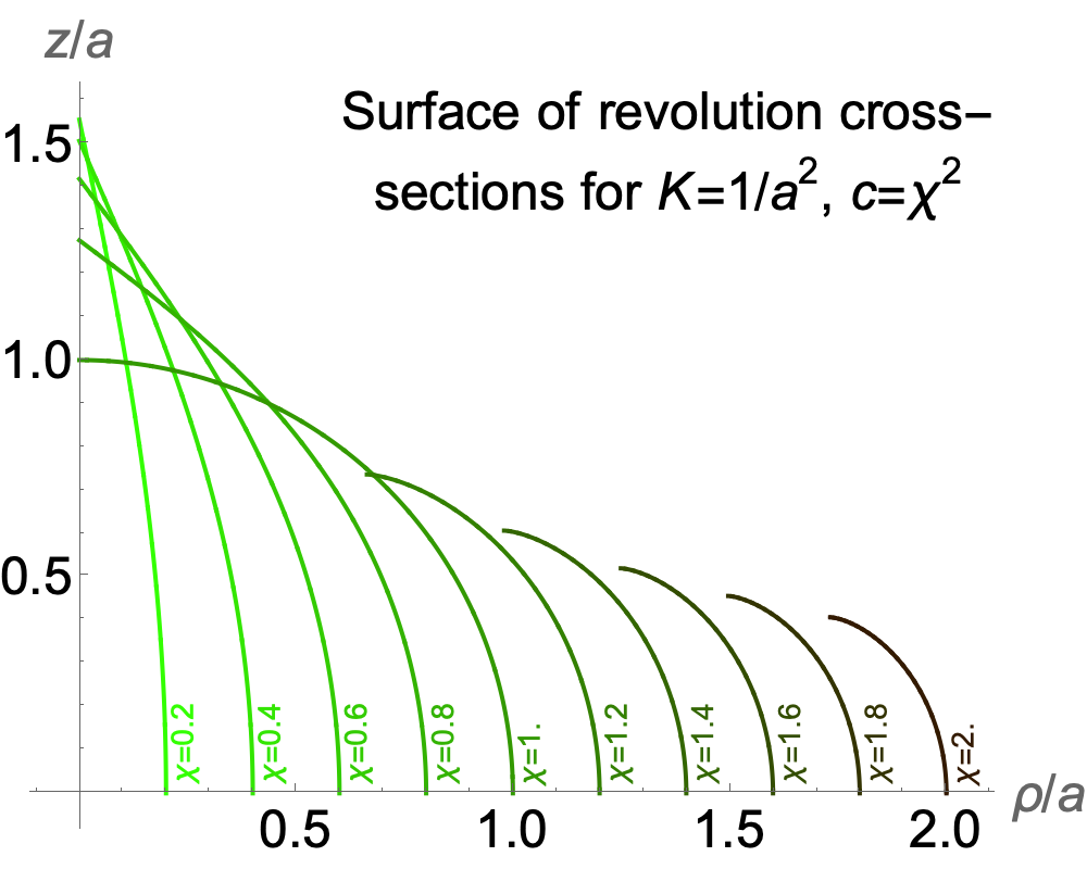
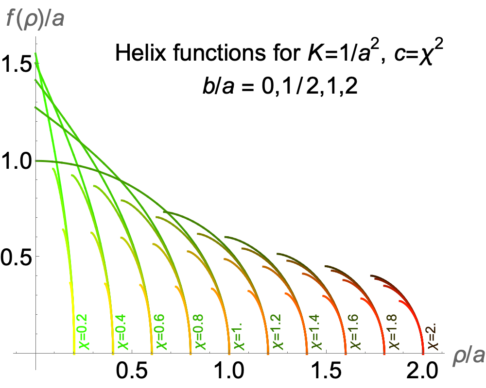
The image on the right shows cross-sections through the surfaces of revolution of constant Gaussian curvature K = 1/a2, for a variety of equatorial radii. Here, c = χ2, and χ is the maximum value of ρ/a for each curve.
These curves all meet the horizontal axis with vertical tangents, so they can be smoothly extended by reflection in this axis; for example, the curve for χ = 1 will yield a complete sphere. However, the points at the top of the curve will (in all other cases besides the sphere) need to be excluded from the surface, with the “poles” for χ < 1 having a local topology like the tip of a cone, and the tops of the curves for χ > 1 giving rise to circular boundaries.
We can compute the lengths of these curves:
L = ∫ρ1ρ2 √[1 + f '(ρ)2] dρ
= ∫ρ1ρ2 1/√[χ2 – (ρ/a)2] dρ
= a arcsin(ρ/(a χ)) |ρ1ρ2
| If 0 < χ ≤ 1 | L = (π/2) a | |
| If χ > 1 | L = (π/2 – arctan(√[χ2 – 1])) a |
So for χ ≤ 1, this is the same as the meridian from the equator to the pole on a sphere of radius a, while for χ > 1 it is shorter.
What about the surface area?
A = 2 π ∫ρ1ρ2 ρ √[1 + f '(ρ)2] dρ
= 2 π ∫ρ1ρ2 ρ/√[χ2 – (ρ/a)2] dρ
= –2 π a √[a2 χ2 – ρ2] |ρ1ρ2
| If 0 < χ < 1 | A = 2 π a2 χ | |
| If χ ≥ 1 | A = 2 π a2 |
For χ < 1, this is less than the hemisphere of a sphere of radius a, while for χ ≥ 1 it is exactly the same.
Now let’s compute geodesics on these surfaces. To start, note that the metric in (φ, ρ) coordinates can be found from our initial calculations, once we substitute the result for f '(ρ):
| g(φ, ρ) | = |
| = |
|
Because the metric is independent of the φ coordinate, we can find a family of geodesics by imposing the requirement that each such curve has a conserved quantity: the dot product of the unit-length tangent to the geodesic and the vector field that corresponds to a uniform increase in the φ coordinate. We won’t go through the derivation, but the results are easily checked. We claim that these curves are geodesics (for c ≠ 0):
Geodesics on generic surface of revolution
φG(s) = φ0 + arctan((√[c/K] / ρ0) tan(s √K)) / √c
ρG(s) = √[ρ02 + (c/K – ρ02) sin2(s √K)]
To verify this, we compute the coordinates of the tangent to the geodesic:
φG'(s) = ρ0 K / (ρ02 K + (c – ρ02 K) sin2(s √K))
ρG'(s) = (c – ρ02 K) sin(s √K) / √[c tan2(s √K) + ρ02 K]
Along these geodesics, the metric becomes:
| g(φG(s), ρG(s)) | = |
|
and we have:
(φG'(s), ρG'(s))T g(φG(s), ρG(s)) (φG'(s), ρG'(s)) = 1
(φG'(s), ρG'(s))T g(φG(s), ρG(s)) (1, 0) = ρ0
This confirms that the tangent has a length of 1, and that its dot product with the φ coordinate vector field is a conserved quantity, the constant ρ0, that parameterises the family of geodesics.
For positive curvature we can write the geodesics as:
Geodesics on positive-curvature surface of revolution
K = 1/a2 c = χ2
Generic case (with s measured from point where ρ = ρ0):
φG(s) = φ0 + arctan((aχ/ρ0) tan(s/a)) / χ
ρG(s) = √[ρ02 + (a2 χ2 – ρ02) sin2(s/a)]
Meridians (with s measured from the equator):
φG(s) = φ0
ρG(s) = a χ cos(s/a)
At s = 0, we have (for both positive and negative curvature):
φG(0) = φ0
ρG(0) = ρ0
φG'(0) = 1/ρ0
ρG'(0) = 0
So at s = 0 the geodesic is tangent to a circle of latitude of radius ρ0, and this is the minimum value of the ρ coordinate for the geodesic. However, for surfaces with χ > 1, if we choose a value for ρ0 that is less than the minimum value for ρ on the entire surface, a √[χ2 – 1], we still obtain a valid geodesic, but it only exists for values of s large enough to give valid values for ρ.
For the positive curvature case, we have:
φG((π/2) a) = φ0 + π/(2 χ)
ρG((π/2) a) = a χ
This tells us that after we travel a distance, (π/2) a, that is the same as the equator-to-pole distance on a sphere of radius a, we arrive at the equator (the maximum value for ρ). The metric in (φ, ρ) coordinates is singular at the equator, but we can calculate the angle between the geodesic and the equator as a limit:
cosine of angle between geodesic and circle of latitude
= dot product between tangent to geodesic and unit vector in the φ direction
= (φG'(s), ρG'(s))T g(φG(s), ρG(s)) (1/ρG(s), 0)
= ρ0 / ρG(s)
cosine of angle between geodesic and equator (ρ = a χ)
= ρ0 / (a χ)
By varying ρ0, we can construct a family of geodesics that all pass through the same point on the equator at various angles.
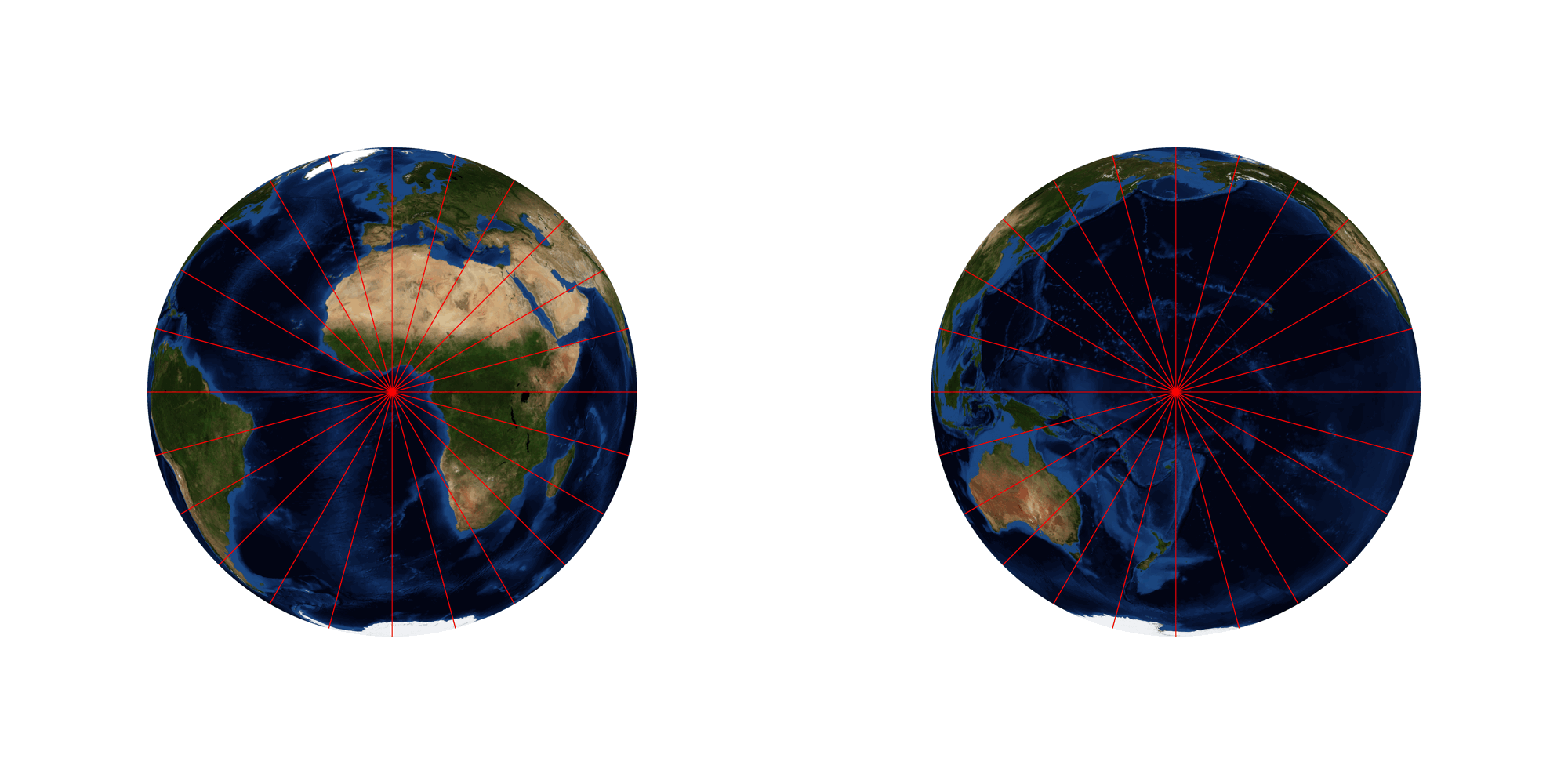
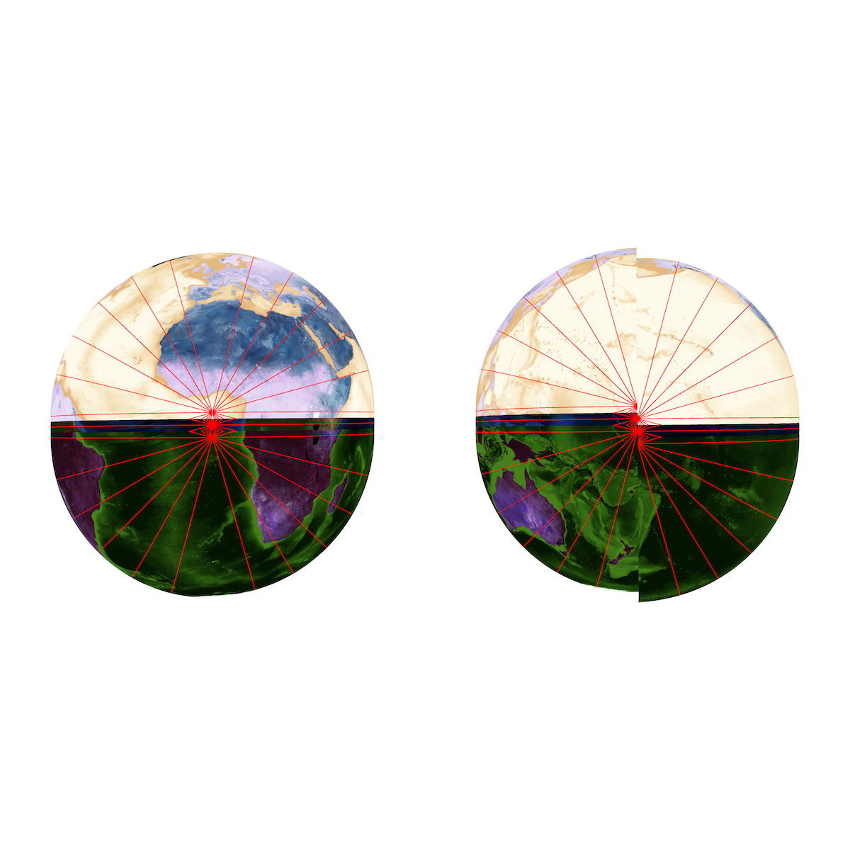
The animation above shows surfaces of revolution, all with the same constant positive curvature, as the parameter χ cycles between 0.5 and 1.5. The two views show the same surface from the front and the back.
The Earth has been mapped to these surfaces by a simple isometry: when χ is less than 1, part of the equator of the Earth, and the full length of each meridian crossing it, is mapped to the equator and meridians on the surface; when χ is greater than 1, the full equator of the Earth, and part of the equator of a second copy of the Earth, and part of each meridian crossing them, is mapped to the equator and meridians on the surface. There is generally a discontinuity in the map along the midline of the view of the surface from behind, but this is not a boundary or singularity in the surface itself. As we mentioned earlier, the poles for the surfaces with χ less than 1 are singular points, in a similar way to the tip of a cone, and need to be excluded. For χ greater than 1 there are two circular boundaries where ρ hits a non-zero minimum value and the surface cannot be extended.
The red curves are geodesics, fanning out from a point on the equator and then reconverging. The geodesics are only drawn until they have gone halfway around the axis, or until they have reconverged, whichever is further. Regardless of the value of χ, the geodesics always reconverge after the same distance, π a, but for χ greater than 1 some of the geodesics hit the boundary of the surface and terminate there. Also, the distance π a will no longer correspond to half the length of the equator, and the second reconvergence, at a distance of 2π a, will no longer take place at the point where we started.
The equator is always a geodesic, but in general geodesics will only form closed loops of finite length when χ is rational, since each portion of a geodesic that lies north or south of the equator will span a longitude of π/χ. And even for rational values of χ, it might take a very large number of crossings of the equator before these changes in longitude sum to an integer multiple of 2π. This leads to the conclusion that, in general, the shortest geodesic path from a point P (not on the equator) that wraps around the surface and returns to P will not be part of a finite loop, which in turn means it must return to P with its tangent pointing in a different direction than when it began. The angle between the tangent to the geodesic and the circle of latitude that P lies on must have the same cosine whenever they cross, so if they are not the same angles, they must be opposites.
So, while the local geometry of these surfaces is exactly like that of a sphere, the global properties are not the same. Insects confined to a surface like this, but able to travel distances comparable to the dimensions of the whole surface, could certainly distinguish it from a sphere by suitable “experiments” with geodesics.
Now let’s consider the case of negative curvature.
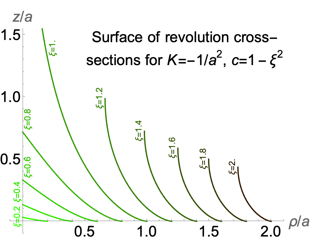
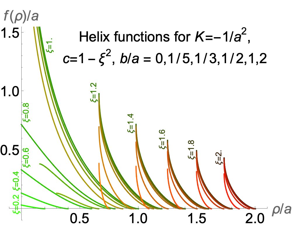
The image on the right shows cross-sections through the surfaces of revolution of constant Gaussian curvature K = –1/a2, for various equatorial radii. We have set c = 1 – ξ2, and ξ is the maximum value of ρ/a for each curve.
All of these curves meet the horizontal axis with a slope of zero, so unlike the case with positive curvature, the surfaces cannot be smoothly extended by reflection here. For ξ < 1, the surfaces will have a conical tip at the point of maximum z; for ξ = 1, the tractrix extends to infinity in the z direction. For ξ > 1, the curves all have a vertical tangent at the minimum radius, ρ = a √[ξ2 – 1], so they can be extended smoothly there by reflection in a horizontal line at the maximum z value.
The lengths of these curves are:
L = ∫ρ1ρ2 √[1 + f '(ρ)2] dρ
= ∫ρ1ρ2 1/√[1 – ξ2 + (ρ/a)2] dρ
= a arctanh(ρ/√[ρ2 + a2(1 – ξ2)]) |ρ1ρ2
| If 0 < ξ ≤ 1 | L = a arctanh(ξ) | |
| If ξ > 1 | L = a arctanh(1/ξ) |
The area of the surface of revolution is:
A = 2 π ∫ρ1ρ2 ρ √[1 + f '(ρ)2] dρ
= 2 π ∫ρ1ρ2 ρ/√[1 – ξ2 + (ρ/a)2] dρ
= 2 π a √[ρ2 + a2 (1 – ξ2)] |ρ1ρ2
| If 0 < ξ < 1 | A = 2 π a2 (1 – √[1 – ξ2]) | |
| If ξ ≥ 1 | A = 2 π a2 |
For ξ < 1 this is less than the hemisphere of a sphere of radius a, while for ξ ≥ 1 it is exactly the same.
For negative curvature we can write the geodesics as:
Geodesics on negative-curvature surface of revolution
K = –1/a2 c = 1 – ξ2
Generic case (with s measured from point where ρ = ρ0):
φG(s) = φ0 + arctan(√[1 – ξ2] (a/ρ0) tanh(s/a)) / √[1 – ξ2]
ρG(s) = √[ρ02 + (ρ02 + a2 (1 – ξ2)) sinh2(s/a)]
Asymptotes to waist (for ξ > 1 only, with s measured from the equator):
φG(s) = φ0 + (½log(1 + (ξ2 – 1) exp(2s/a)) – log(ξ)) / √[ξ2 – 1]
ρG(s) = a √[ξ2 – 1 + exp(–2s/a)]
Meridians:
φG(s) = φ0
- for ξ < 1 (with s measured from the pole):
ρG(s) = a √[1 – ξ2] sinh(s/a)- for ξ > 1 (with s measured from the “waist”):
ρG(s) = a √[ξ2 – 1] cosh(s/a)
We can also compute the special case c = 0, ξ = 1, for geodesics on the tractroid:
Geodesics on tractroid
K = –1/a2 c = 0
Generic case (with s measured from point where ρ = ρ0):
φG(s) = φ0 + (a/ρ0) tanh(s/a)
ρG(s) = ρ0 cosh(s/a)
Meridians (with s measured from the equator):
φG(s) = φ0
ρG(s) = a exp(–s/a)
Polar geodesic coordinate systems
If we pick a point on the tractroid, say (ρ, φ) = (ρC, φC),
we can construct a set of geodesics that all pass through
that point, and whose tangents at that point are parameterised
by an angle θ:
φG(s) = φC + a cos(θ) sinh(s/a) / [ρC (cosh(s/a) – sin(θ) sinh(s/a))]
ρG(s) = ρC (cosh(s/a) – sin(θ) sinh(s/a))
The arc length parameter s is measured from the chosen point,
and the angle θ is measured from a horizontal tangent.
As with the positively curved surfaces, in the generic case these geodesics are tangent, at s = 0, to a circle of latitude of radius ρ0, and this is the minimum value of the ρ coordinate for the geodesic. If ξ > 1 and we choose ρ0 to be less than the minimum value for ρ on the entire surface, a √[ξ2 – 1], we still obtain a valid geodesic, but it only exists for values of s large enough to give valid values for ρ.
However, unlike the positive curvature case, all geodesics on a given surface do not take the same distance from their point of minimum ρ before they reach the equator. And the equator itself is not a geodesic; its geodesic curvature (the curvature in terms of the intrinsic geometry, relative to the geodesics, which are considered to be straight) is the same as its curvature in three-dimensional Euclidean space: 1/(a ξ), the reciprocal of the radius of the equatorial circle.
For ξ ≤ 1, most geodesics will start and end on the equator. Meridians will start on the equator and end on the pole, or for ξ = 1 will continue to infinity.
For ξ > 1, the surface has a “waist,” a circle of minimum ρ where ρ = a √[ξ2 – 1]. This is clearly a geodesic by symmetry, and if we insert this value for ρ0 into the formula for the generic ρG(s), it becomes constant. Geodesics with ρ0 < a √[ξ2 – 1] will cross the waist, and have endpoints on the two distinct copies of the equator. Geodesics with ρ0 > a √[ξ2 – 1] will never cross the waist, and will start and end on the same copy of the equator. Geodesics with ρ0 = a √[ξ2 – 1] that do not start on the waist are asymptotic to it.
As before, the cosine of the angle between a geodesic and any circle of latitude will be equal to ρ0 / ρG(s), so the cosine of the angle between a geodesic and the equator is ρ0 / (a ξ). For ξ > 1 the geodesics that cross the waist will be those that make angles greater than arccos √[1 – 1/ξ2] with the equator. If a geodesic leaves the equator at precisely this angle, it will approach the waist asymptotically, never reaching it but also never returning to the equator.
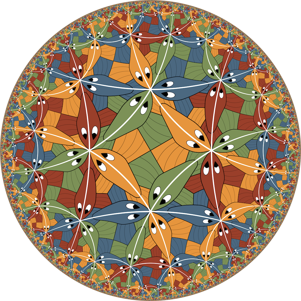
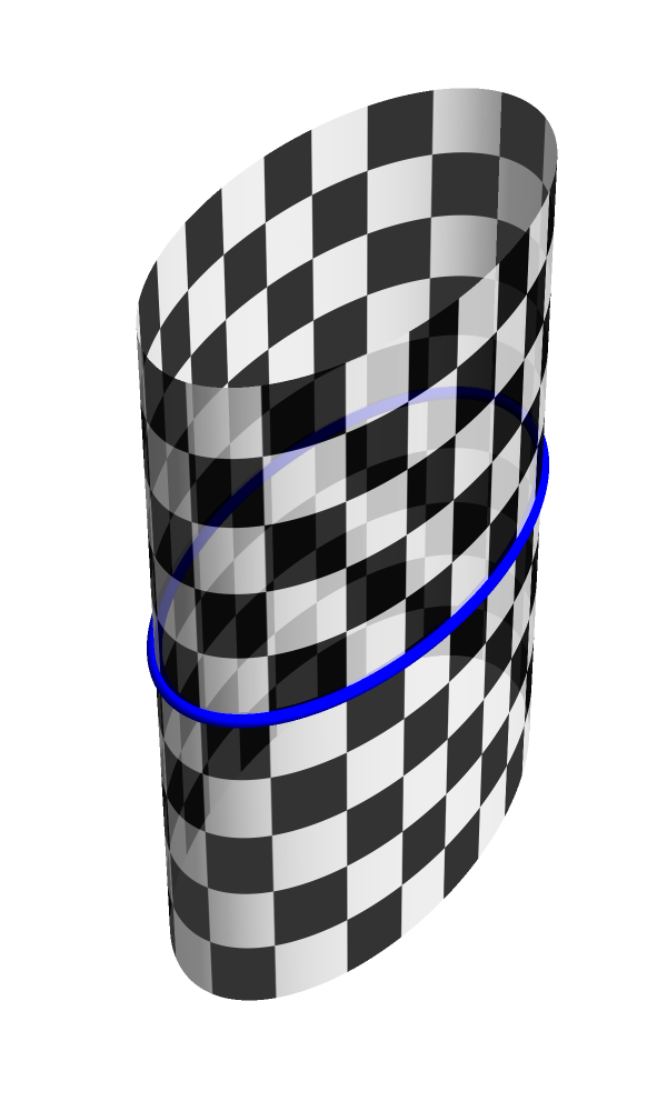
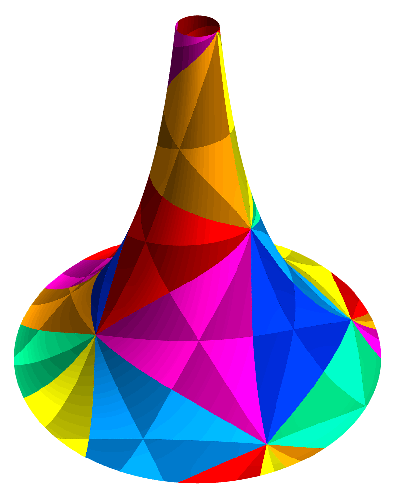
The animation above shows front and back views of surfaces of revolution with K = –1, with the parameter ξ ranging from 1.10125 to 1.70728. These values have no special significance in terms of the properties of the surface, but they were chosen so that the particular tiling of the hyperbolic plane used to illustrate the surface wraps around neatly at the two endpoints. In this tiling, seven equilateral triangles meet at a point, and the equilateral triangles are further subdivided into six right-angled triangles. This tiling can’t exist in the Euclidean plane, where the angles at each vertex of an equilateral triangle are always π/3 radians, but in the hyperbolic plane the sum of the angles of a triangle will be less than π by an amount that depends on the area of the triangle, as we discussed earlier. For these equilateral triangles with angles of 2π/7 at each vertex, for a total of 6π/7, the area is π/7.
The total area of each of the surfaces in the animation is 4π. The isometries used to map the hyperbolic plane to these surfaces take a fixed geodesic in the hyperbolic plane to the circle around the waist of the surface, and then map geodesics orthogonal to the first one to meridians on the surface.
The images on the left and below show some examples of these surfaces rotating, to give a clearer sense of how the negatively curved geometry fits into three-dimensional Euclidean space.
The animation above shows surfaces with K = –1 and the parameter ξ ranging from (√13)/7 ≈ 0.515 to (√45)/7 ≈ 0.958. Each surface corresponds to a circular wedge of the hyperbolic plane, with a wedge angle of 2 π √[1 – ξ2], a radius of arctanh(ξ), and a total surface area of 2 π (1 – √[1 – ξ2]). The wedge angles here range from 6 × 2π/7 to 2 × 2π/7, as can be seen by the numbers of triangles from the tiling that fit around the pole.
The tractroid, with ξ = 1, can be viewed as a limiting case of this family of conelike surfaces, where the height of the cone goes to infinity while the wedge angle goes to zero, in such a way that the total area of the surface remains finite at 2π a2. Because the distance from the pole to the equator goes to infinity, any real-world example of the tractroid will just be a portion of the whole surface, in the vicinity of the equator rather than the pole.
The equator of the tractroid is not a geodesic; it corresponds to a finite portion of an infinite curve in the hyperbolic plane known as a horocycle, which can be thought of as a kind of circle whose centre lies, not in the hyperbolic plane itself, but “at infinity.” In hyperbolic geometry, a point like this is known as an ideal point. In the Poincaré disk model of the hyperbolic plane, the plane is represented by the interior of a disk, while the ideal points lie on the boundary of the disk, and horocycles are represented by circles that are tangent to the boundary circle.
The meridians of the tractroid are geodesics, meeting the horocycle of the equator orthogonally, and converging on a common ideal point. Because there are no pairs of geodesics from the edges in our tiling that converge on an ideal point, there is necessarily a visible “seam” in the pattern along one meridian of the tractroid in the image on the right.
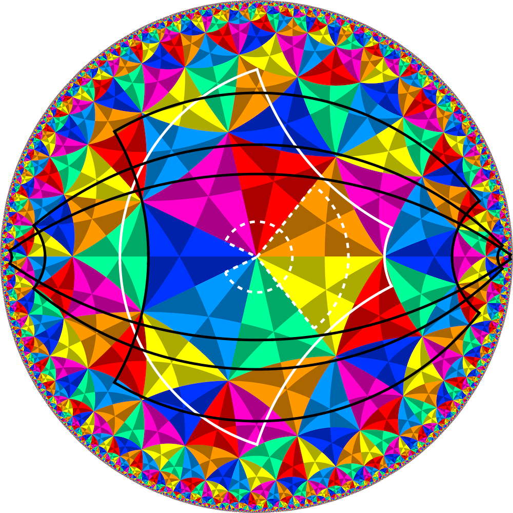
The image on the left shows the outlines of regions of the hyperbolic plane, in the Poincaré disk model, that are mapped to the negatively curved surfaces we have illustrated.
The dashed white shapes are the two extremes of the wedges mapped to the cone-like surfaces with ξ < 1.
The solid white line shows the region mapped to the tractroid. The large arc on the left, corresponding to the equator of the tractroid, is part of a horocycle; the small arc on the right, corresponding to the circle of latitude where we chose to truncate the tractroid, is part of another horocycle.
The black shapes are three regions mapped to the hourglass-like surfaces with ξ > 1. The curves that cross the x-axis are geodesics, corresponding to meridians of the hourglass, while the upper and lower boundaries are hypercycles (curves at a fixed distance from a geodesic, in this case the x-axis), corresponding to the circles of latitude of maximum ρ. The x-axis itself corresponds to the waist of the hourglass.
In the previous section, we constructed surfaces of revolution composed of circles of varying radius, ρ, with their z coordinate (their location along the axis of revolution) given by a function, f(ρ), which satisfied a differential equation that ensured constant Gaussian curvature.
One way to generalise this construction, while still working with just one function of a single variable, is to replace all the circles with helices of a specified pitch, controlled by a parameter b that is a constant for each surface. The parameterisation of the surface then takes the form:
x(φ, ρ) = (ρ cos φ, ρ sin φ, f(ρ) + b φ)
The surfaces of revolution correspond to b = 0. Computing the Gaussian curvature:
xφ = (–ρ sin φ, ρ cos φ, b)
xρ = (cos φ, sin φ, f '(ρ))
n = xφ × xρ / |xφ × xρ| = (ρ f '(ρ) cos φ – b sin φ, b cos φ + ρ f '(ρ) sin φ, –ρ) / √[b2 + ρ2 (1 + f '(ρ)2)]
xφφ = (–ρ cos φ, –ρ sin φ, 0)
xφρ = (–sin φ, cos φ, 0)
xρρ = (0, 0, f ''(ρ))
g(φ, ρ) =
xφ · xφ xφ · xρ xφ · xρ xρ · xρ =
ρ2 + b2 b f '(ρ) b f '(ρ) 1 + f '(ρ)2 S(φ, ρ) =
xφφ · n xφρ · n xφρ · n xρρ · n =
–ρ2 f '(ρ) / √[b2 + ρ2 (1 + f '(ρ)2)] b / √[b2 + ρ2 (1 + f '(ρ)2)] b / √[b2 + ρ2 (1 + f '(ρ)2)] –ρ f ''(ρ) / √[b2 + ρ2 (1 + f '(ρ)2)]
K = det(S) / det(g) = (ρ3 f '(ρ) f ''(ρ) – b2) / (b2 + ρ2 (1 + f '(ρ)2))2)
We can rewrite this differential equation in f as:
q(ρ) = (b2 + ρ2 (1 + f '(ρ)2))–1
–½ ρ q'(ρ) – q(ρ) = K
which is solved by:
q(ρ) = c / ρ2 – K
f '(ρ) = ±√[1/(–K ρ2 + c) – (1 + b2/ρ2)]
Here c is a constant of integration, and the result for f '(ρ) agrees with that for a surface of revolution if we set b = 0.
For the quantity inside the square root to be finite and non-negative we need:
0 < –K ρ2 + c < ρ2 / (ρ2 + b2)
and ρ > 0
The right-hand inequality in the first line above becomes an equality when ρ2 is a root of the equation:
K (ρ2)2 + (K b2 – c + 1) ρ2 – b2 c = 0
In everything that follows, we will assume that b > 0. For the case of positive curvature, we will set K = 1/a2 and c = χ2, since we need c > 0 in order to have a non-empty range for ρ:
½(d + √[d2 + 4 a2 b2 χ2]) < ρ2 < (a χ)2
where d = a2 (χ2 – 1) – b2
So we have the same maximum value for ρ as for the positive-curvature surfaces of revolution, but now we always have a non-zero minimum value for ρ, regardless of the value of χ. The derivative f '(ρ) approaches infinity at the outer limit for ρ, and zero at the inner limit.
For negative curvature, we will set K = –1/a2 and c = 1 – ξ2, since we need c < 1 in order to have a non-empty range for ρ:
If 0 < ξ ≤ 1 and
b < a (1 – √[1 – ξ2])½(d – √[d2 + 4 a2 b2 (ξ2 – 1)]) < ρ2 < ½(d + √[d2 + 4 a2 b2 (ξ2 – 1)]) If ξ > 1 a2 (ξ2 – 1) < ρ2 < ½(d + √[d2 + 4 a2 b2 (ξ2 – 1)])
where d = a2 ξ2 – b2
In the first case, f '(ρ) is zero at two positive roots for ρ2, and the upper bound we have placed on b is needed in order for those roots to be real and positive. In the second case, f '(ρ) approaches infinity at the inner limit for ρ, and zero at the outer limit.
In general we will have a non-zero minimum value for ρ, but if ξ = 1 the limits become:
If ξ = 1 and b < a 0 < ρ2 < a2 – b2
We will integrate f '(ρ) first for the special case ξ = 1 (i.e. c = 0). This yields a tractroid when b = 0, and in fact the integral is identical apart from changing the constant a in the previous formula to √[a2 – b2]:
Dini’s surface
K = –1/a2 c = 0 b < a ρm = √[a2 – b2]
f '(ρ) = ±√[ρm2 – ρ2] / ρ
f(ρ) = zρm ± (√[ρm2 – ρ2] – ρm arccosh(ρm/ρ))
The result we obtain by substituting this solution into our parameterisation of helical surfaces is known as Dini’s surface.
Note that the parameterisations for this family of surfaces in the literature can look very different from the one we have used. For example, MathWorld gives the parameterisation:
(x, y, z) = (a cos u sin v, a sin u sin v, a [cos v + log(tan ½v)] + b u)
which has a Gaussian curvature of –1/(a2 + b2) rather than –1/a2, and while u here is the same as our φ, the coordinate v is analogous to the colatitude θ in spherical polar coordinates, and our ρ coordinate is proportional to sin v. But if we replaced a here with √[a2 – b2] this would describe exactly the same surface as ours.
Because the metric for all the surfaces built from helices is independent of the φ coordinate, as it was for the surfaces of revolution, we again have a conserved quantity along each geodesic: the dot product between the unit-length tangent to the geodesic and the vector (1,0), which represents a uniform change of φ. The difference is that, this time, rather than pointing around in a circle, the vector for a change in φ points along the helices from which the surface is built.
For Dini’s surface, the formulas for ρ in the geodesics take a very similar form to that of geodesics on the tractroid, but the formulas for φ are considerably more complicated. We don’t really have “meridians” anymore, but the geodesics can be grouped into three classes: those which have a minimum ρ value, ρ0 > 0, those where ρ is only bounded below by zero, and are of finite length, and those which are of infinite length and approach ρ = 0 asymptotically.
Geodesics on Dini’s surface
K = –1/a2 c = 0 b < a ρm = √[a2 – b2]
Geodesics with lower bound ρ0 on ρ (with s measured from the point where ρ = ρ0):
ρG(s) = ρ0 cosh(s/a)
φG(ρ) = φ0 + (ρm/b) log( (ρm + √[ρm2 – ρ2]) (ρm – √[ρm2 – ρ02]) / (ρ ρ0))
+ ½ (a/b) log(
(a – √[ρm2 – ρ2]) (a + √[ρm2 – ρ02]) (ρ02 + b (b – √[b2 + ρ02])) (ρ (ρ – √[ρ2 – ρ02]) + (b (b + √[b2 + ρ02]))) /
[(a + √[ρm2 – ρ2]) (a – √[ρm2 – ρ02]) (ρ02 + b (b + √[b2 + ρ02])) (ρ (ρ – √[ρ2 – ρ02]) + (b (b – √[b2 + ρ02])))] )
The angle between the geodesic and the helix ρ = ρm is acos(√[b2 + ρ02]/a).
Geodesics where ρ goes to zero in a finite distance (with s measured from the point where ρ = ρm):
ρG(s) = ρm cosh(s/a) – √[a2 – γ2] sinh(s/a)
φG(ρ) = φ0 + (ρm/b) arctanh(√[1 – (ρ/ρm)2]) – (a/b) arccoth(a/√[ρm2 – ρ2])
– ½ (a/b) log(
(ρm √[a2 – γ2] + b γ – a2) (b (b + γ) + ρ (ρ – √[ρ2 + b2 – γ2])) /
[(ρm √[a2 – γ2] – b γ – a2) (b (b – γ) + ρ (ρ – √[ρ2 + b2 – γ2]))] )
Here γ is a parameter, 0 < γ < b. The angle between the geodesic and the helix ρ = ρm is acos(γ/a).
Geodesics where ρ goes to zero asymptotically (with s measured from the point where ρ = ρm):
ρG(s) = ρm exp(–s/a)
φG(ρ) = φ0 + (a/b) log(ρm(a – √[ρm2 – ρ2])/(a ρ)) + (ρm/b) log((ρm + √[ρm2 – ρ2])/ρ)
The angle between the geodesic and the helix ρ = ρm is acos(b/a).
It might be a bit surprising, at first, to realise that there are geodesics on Dini’s surface that travel between the outer helix, with ρ = ρm, and points where ρ = 0, in a finite distance. On the tractroid, the equator lies at one end of an infinitely long funnel that takes an infinite distance to taper down to zero width. But although there is a contribution to the z coordinate of Dini’s surface that grows infinitely negative as ρ approaches zero, these finite-length geodesics counterbalance that with the contribution from φ approaching positive infinity, so they terminate at a finite value for z.
We can measure the width of Dini’s surface by the length of the orthogonal geodesics between the outer helix ρ = ρm and the line ρ = 0; these are the geodesics where we set γ = 0, and their length is a arccosh(a/b). The surface can be continued infinitely far in the positive and negative φ directions, along the helices.
We can construct an isometry between Dini’s surface and an infinitely long strip within the hyperbolic plane, bounded on one side by a geodesic, and on the other by a hypercycle, a curve that lies at a fixed distance from that geodesic. The hypercycle corresponds to the outer helix of Dini’s surface, and the geodesic corresponds to the line ρ = 0. In the Poincaré disk model, a hypercycle is represented by a circular arc that meets the boundary of the disk at the same points as its associated geodesic, while the geodesic itself is either a diameter of the disk, or a circular arc that meets the boundary orthogonally.
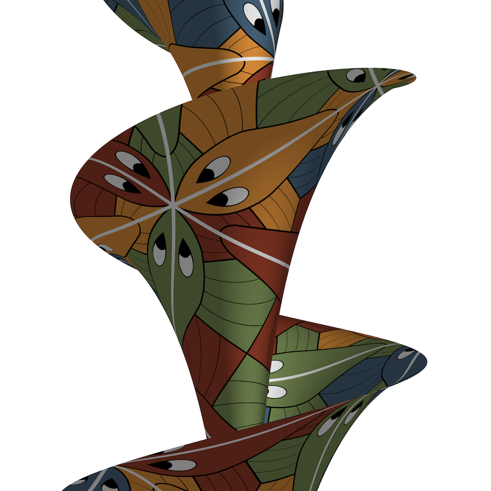
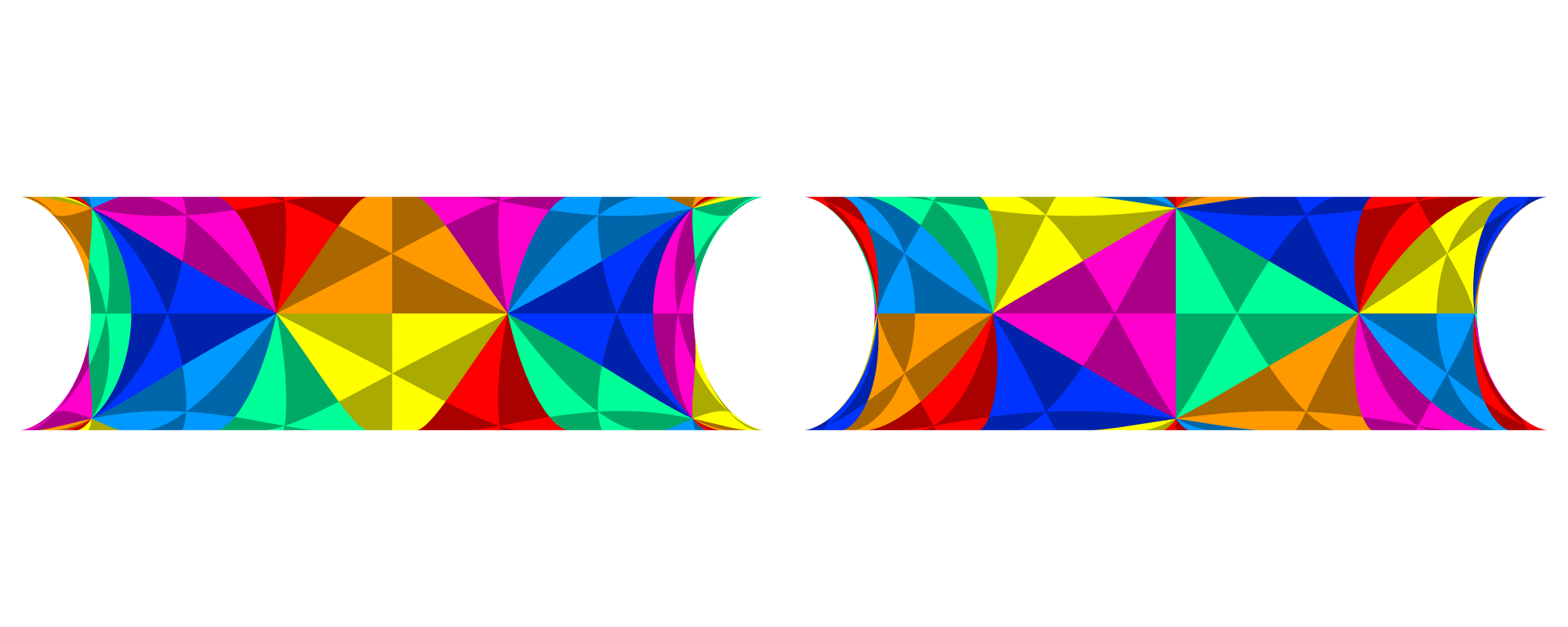
The image on the right shows a finite piece of Dini’s surface, with a = 1, b = 1/4 and –3π ≤ φ ≤ 3π along the outer helix. We have cut the surface along two geodesics orthogonal to the outer helix, but to be clear, these are not lines of constant φ. The isometry that we’ve used here maps the x-axis of the Poincaré disk model to the line ρ = 0, while the outer helix on the surface corresponds to a circular arc in the upper half of the Poincaré disk that passes through the points (–1, 0), (0, √[(1–b)/(1+b)]) and (1, 0). The tiling is the same one we used for all the negatively-curved surfaces in the previous section.
The image on the left shows how the shape of Dini’s surface changes as we vary b, which cycles here between 1/12 and 1/4. For a given range of φ (measured along the outer helix), the surface area is equal to Δφ √[1–b2], so as the pitch of the helices decreases, the area increases. The precise shape of the corresponding region in the hyperbolic plane changes too; while the length of the arc of the hypercycle remains equal to Δφ, the length of the portion of the geodesic along the x-axis at the bottom of the region is Δφ b, while the length of the geodesics joining those two boundaries is arccosh(1/b).
In the limit as b approaches zero, each loop of the outer helix of Dini’s surface approaches the same arc of a horocycle as the equator of the tractroid. But so long as b does not actually reach zero, we can continue to include as many loops as we wish without the surface self-intersecting.
It’s impossible to embed the entire hyperbolic plane in three-dimensional Euclidean space, but the parameters for Dini’s surface can be chosen so that it contains a disk of any finite radius R, while its Gaussian curvature remains fixed at –1. If we set:
a = 1
b = 1/cosh(2R)
Δφ = 2 cosh(2R) arccosh(√[1 + tanh2(R)])
then a disk of radius R will fit inside the surface, with the outer helix, the centreline, and the orthogonal geodesics that leave the outer helix at the minimum and maximum values of φ, all being tangent to the disk.
 |
 |
We will now consider the general case of a surface of constant Gaussian curvature constructed from helices, where c ≠ 0 and b ≠ 0. Although it is possible to write down a closed form for the function f(ρ) in terms of elliptic integrals, the expression is so complicated that it is not very enlightening, and it is generally more practical to use direct numerical integration of f '(ρ) to construct the solution.
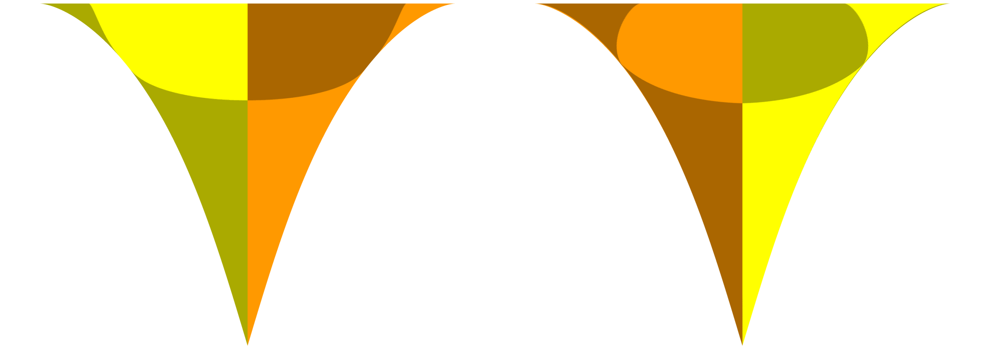
The two plots on the right give examples of f(ρ) for positive and negative curvature, respectively. The green component of each curve’s colour is determined by the value of the parameter we use to set c, while the red component depends on b.
For positive curvature (top right), the maximum value of ρ/a is χ, so it is independent of b, and each family of curves where χ is fixed and b varies meet the horizontal axis at the same point. Increasing b results in a larger lower bound on ρ, shrinking the overall range of values for ρ, and also a lower maximum value for f(ρ).
All of these curves are vertical (i.e. f '(ρ) is infinite) at their maximum value of ρ, so they can be smoothly extended by reflection in the horizontal axis.
For negative curvature (bottom right), the curves with ξ ≥ 1 all share a common minimum value for ρ/a of √[ξ2 – 1], while the maximum value for ρ/a starts at ξ when b = 0 but then falls as b increases. The curves with ξ > 1 become vertical at their minium ρ value, so as with the hourglass-shaped surfaces of rotation we can smoothly extend them by reflection in a horizontal line through that point.
For curves with ξ < 1 both the minimum and maximum values of ρ depend on b as well as ξ, but there is also a ξ-dependent upper bound on the allowed values for b/a of:
b/a < 1 – √[1 – ξ2]
For ξ = 0.8 this bound is 0.4, so there are three curves plotted, for b/a equal to 0, 1/5 and 1/3. For the lower values of ξ, only b = 0 is plotted.
No curves with ξ < 1 are vertical at either endpoint, so they cannot be extended by reflection.
In all cases, increasing b shrinks the range of values for ρ, and in almost all cases it also lowers the maximum value for f(ρ). The only exception is when ξ = 1, which is Dini’s surface, where f(ρ) goes to infinity as ρ approaches zero.
To set up isometries between these helical surfaces and the sphere or hyperbolic plane, it is helpful to know the geodesic curvature, κg, of the helices. This can be computed as the scalar triple product between the unit-length tangent to the helix, t(s), its rate of change with respect to arc length along the helix, t'(s), and the unit normal to the surface[3]. This turns out to be:
κg = √[(c – K ρ2) / (b2 + ρ2)]
Note that when the numerator here is zero, the derivative f '(ρ) of the helix function is infinite, which occurs at the maximum value of ρ for all surfaces of positive curvature, and the minimum value of ρ for surfaces of negative curvature with ξ>1. So in those cases, the widest or narrowest helix on the surface is a geodesic.
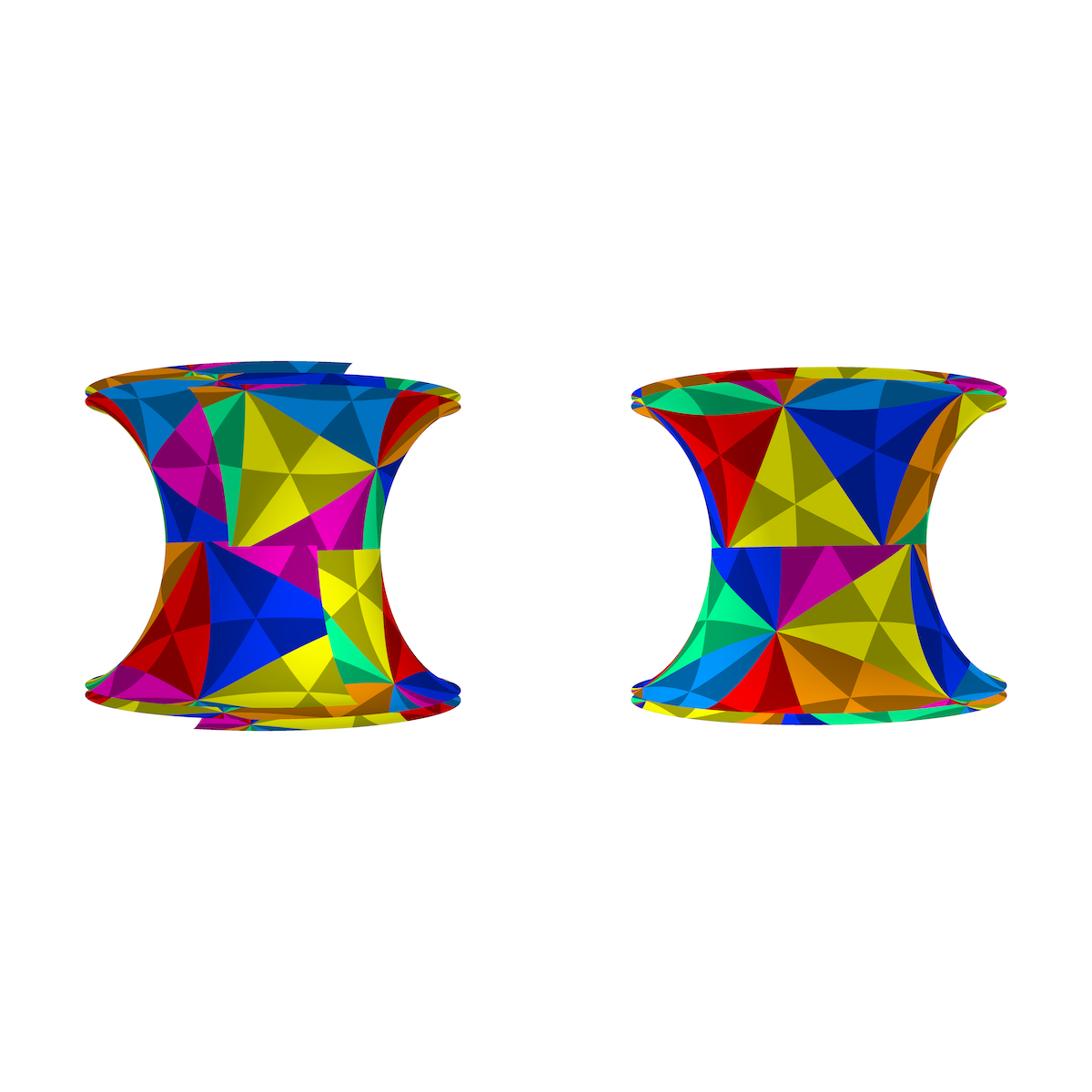
The image above shows parts of the surfaces of constant positive curvature with a = 1, χ = 1, and b ranging from 0.01 to 0.5, as seen from two opposite viewpoints. In each case the surface consists of portions of three copies of the sphere, with the full length of the equator of all three spheres joined together to form the “equatorial helix” (the helix of maximum ρ), while the range of latitude varies depending on the value of b.
For low values of b, the surface is self-intersecting. The critical value for b occurs when:
|f(ρmax) – f(ρmin)| = π b
For a = 1, χ = 1, this can be found numerically to be bcrit ≈ 0.2629.
The red curves in the image are geodesics fanning out from a single point on the equatorial helix, some of which hit the boundary of the surface along helices corresponding to circles of latitude, while others reconverge in the usual manner, after integer multiples of the distance π a. Because of the symmmetry of the situation, the bundle of geodesics that avoid hitting the boundary the first time will continue to do so, and on the idealised version of the surface that continues indefinitely, they will reconverge an infinite number of times at different points. For the lowest value of b at which the surface is non-self-intersecting, a fan of geodesics about 116° wide centred on the equatorial helix will reconverge without hitting the boundary.
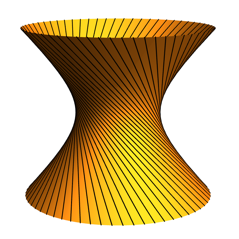
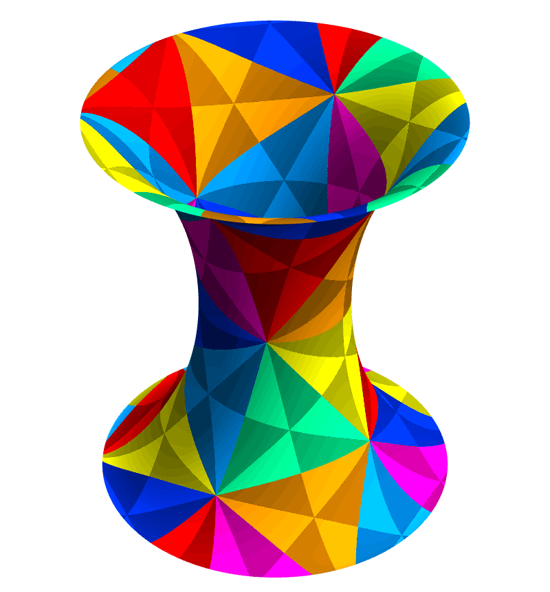
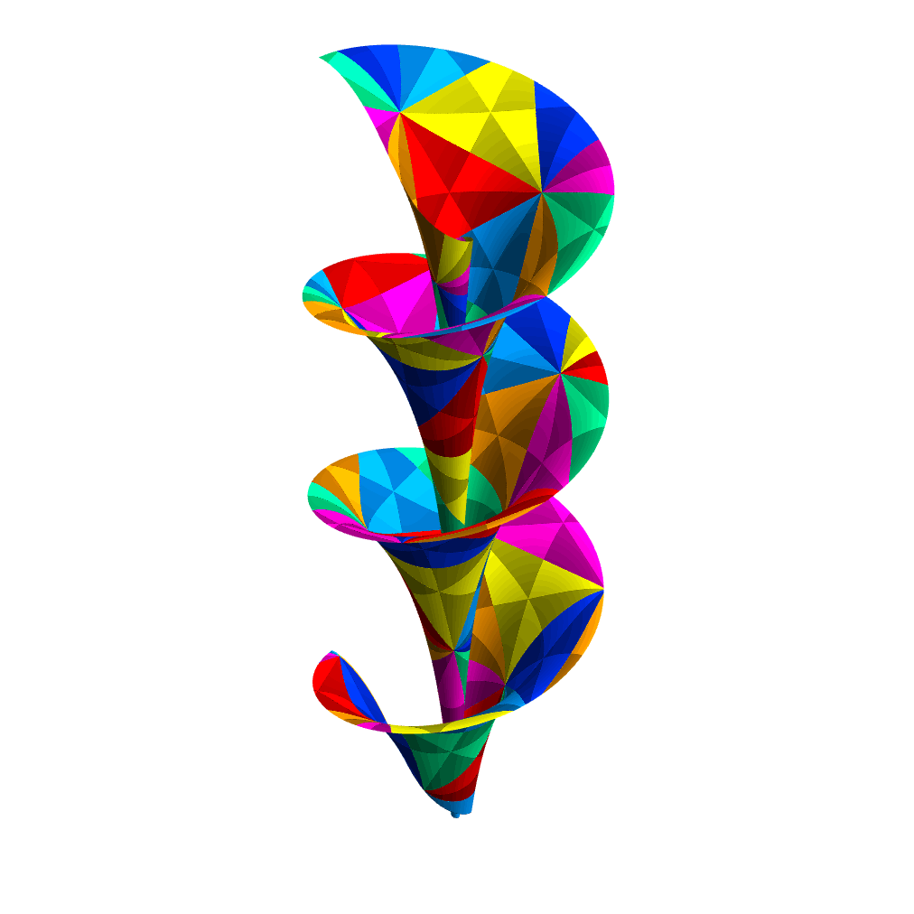
The image above shows parts of the surfaces of constant negative curvature with a = 1, ξ = √[3/2] (i.e. c = 1 – ξ2 = – ½), and b ranging from 0.01 to 0.5, as seen from two opposite viewpoints. Here we have held the total length of the centreline of the ribbon constant, but the width of the ribbon in each case is the maximum possible, which becomes slightly less as b increases.
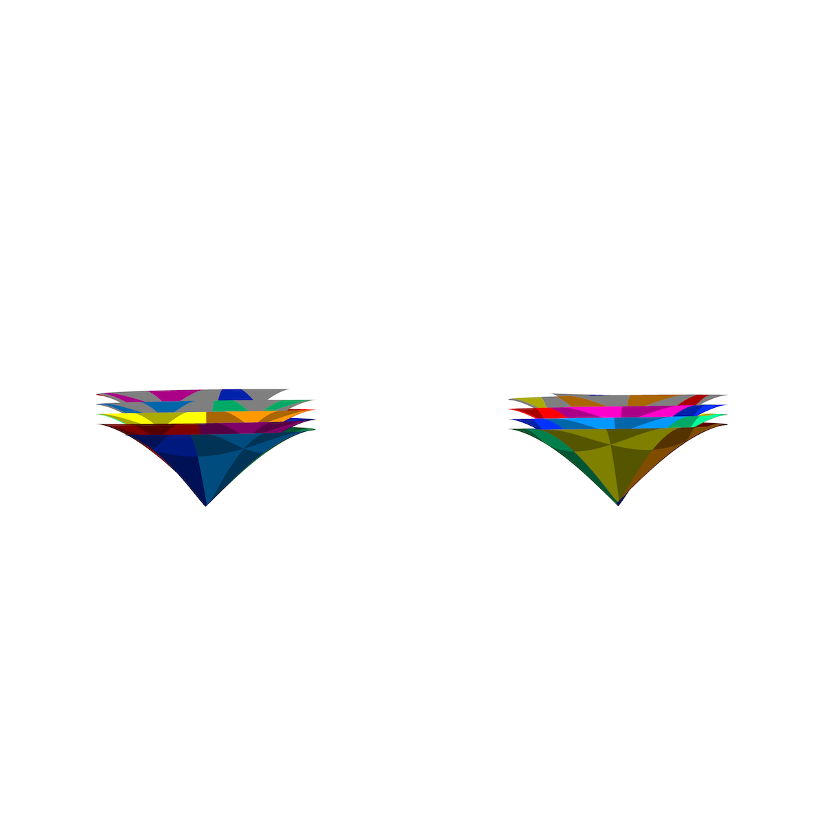
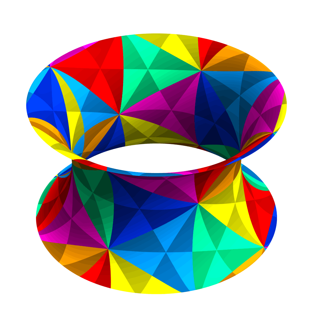
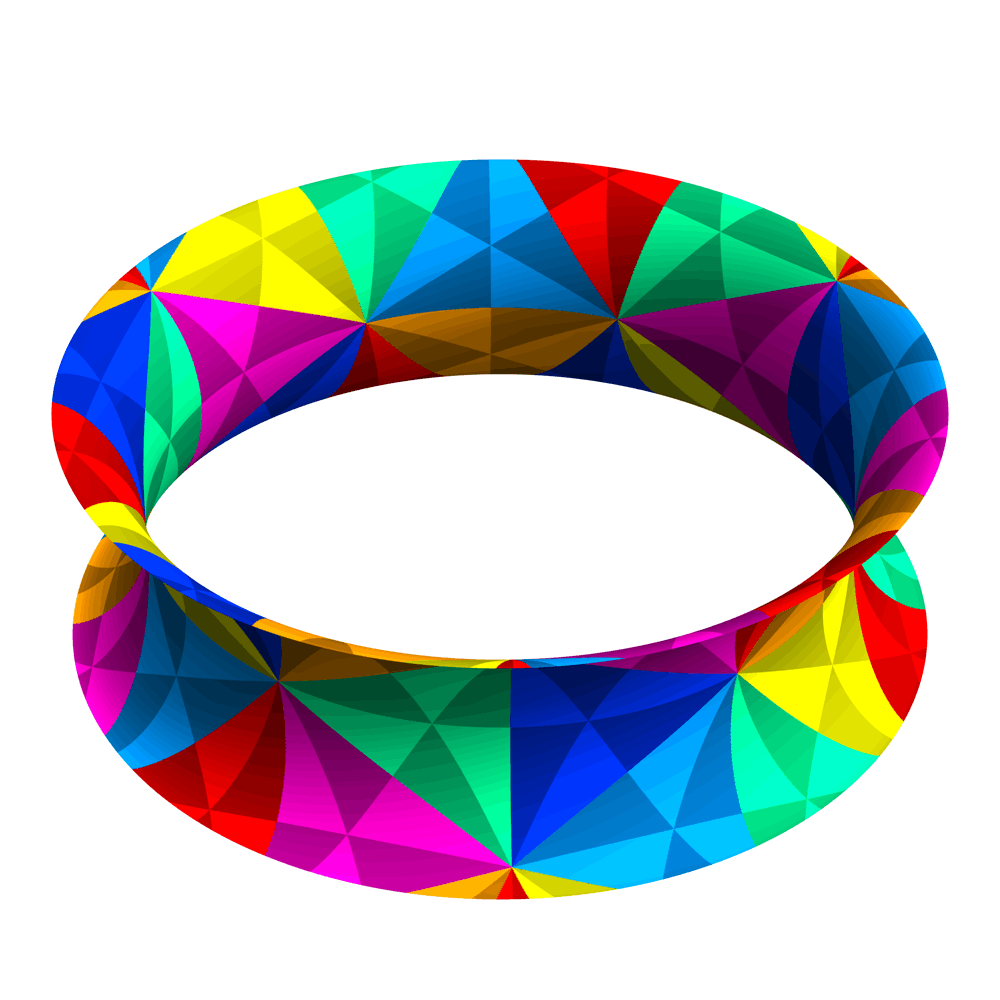
Finally, if K is negative and 0 < c < 1, we get a helical version of the cone-shaped surfaces we obtained for the same parameters when b = 0. The image above shows parts of the surfaces of constant negative curvature with a = 1, ξ = √[1/2] (i.e. c = 1 – ξ2 = ½), and b ranging from 0.01 to 0.292893, as seen from two opposite viewpoints. This ribbon corresponds to an annulus in the hyperbolic plane, and although we can extend its length indefinitely, we will need multiple copies of the hyperbolic plane (illustrated here by changing the shading of the triangular tiling), as any isometry will identify different portions of the ribbon with the same annulus. Here, we show the ribbon obtained from exactly three copies of the annulus.
As with the other helical surfaces, increasing b shrinks the width of the ribbon, but in this case there is a finite upper bound on b of a(1 – √c), at which the width reaches zero.
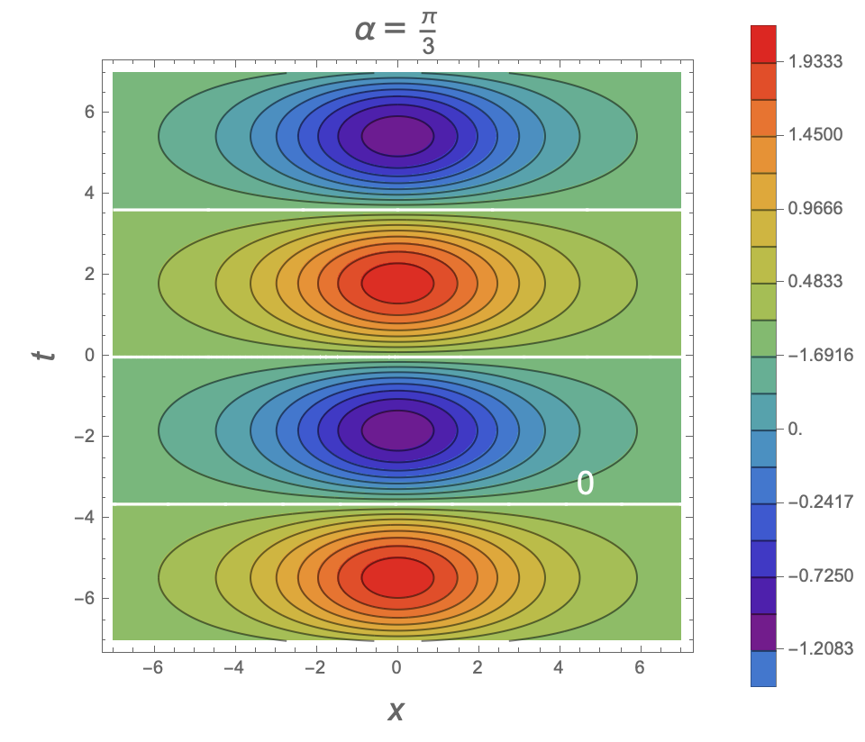
Suppose we have a surface with coordinates u, v that have been chosen so that the metric for the surface takes the form:
g(u, v) =
1 cos(ω(u, v)) cos(ω(u, v)) 1
where ω(u, v) is some as yet unspecified function of the coordinates, and for now we just require that it obeys 0 < ω(u, v) < π in the region of the surface of interest to us. Geometrically, ω(u, v) measures the angle between the curves of the coordinate grid, where we hold u constant and vary v, or vice versa. The diagonal components of the metric being 1 means that the coordinate values along these grid lines are actual distances.
If we compute the Gaussian curvature of the surface, using the method described in the appendix, this turns out to be:
K(u, v) = –∂u,vω(u, v) / sin(ω(u, v))
If the surface has a constant Gaussian curvature K, this gives us partial differential equation that ω(u, v) must satisfy:
∂u,vω(u, v) = –K sin(ω(u, v))
The equation for K = –1:
The sine-Gordon equation
∂u,vω(u, v) = sin(ω(u, v))
is known as the sine-Gordon equation. (The current name for this equation is a pun on another equation, the Klein–Gordon equation, which was actually named much later. The sine-Gordon equation was first studied in the 1860s by Edmond Bour, in relation to surfaces of constant negative curvature, whereas the Klein–Gordon equation was developed in 1926, and describes the wave function of a relativistic particle with zero spin.)
Before searching directly for solutions of the sine-Gordon equation, we should check if any solutions are hiding in the surfaces of constant curvature we have already studied. We haven’t seen any metrics of the form shown above, but there is a way of taking a metric in coordinates x, y that is diagonal and depends only on one coordinate, say y, and obtaining new coordinates in which the metric has diagonal components of 1.
Suppose we are able to find a function F(s) that satisfies the following equation, where g(y) is the metric on the surface as a function of the y coordinate:
(1, F '(s))T g(F(s)) (1, F '(s)) = L2
Because the metric is diagonal, the left-hand side, when multiplied out, only involves F '(s)2, so it will also be true that:
(1, –F '(s))T g(F(s)) (1, –F '(s)) = L2
Now, define new coordinates on the surface, u, v, such that:
x(u, v) = (u + v)/L
y(u, v) = F((u – v)/L)
This gives us:
∂u (x(u, v), y(u, v)) = (1 / L, F '((u – v)/L) / L)
∂v (x(u, v), y(u, v)) = (1 / L, –F '((u – v)/L) / L)
The metric then has diagonal components in the new coordinates of:
guu = 1
gvv = 1
We can apply this method to the metric for the tractroid in (φ, ρ) coordinates, which depends only on the ρ coordinate:
g(ρ) =
ρ2 0 0 1 + f '(ρ)2 =
ρ2 0 0 a2 / ρ2
This gives us the equation for F(s):
F(s)2 + a2 F '(s)2 / F(s)2 = L2
If we set L = 1 and a = 1, this is solved by:
F(s) = sech(s + C)
F '(s) = –sech(s + C) tanh(s + C)
We then have :
ρ = F(u – v)
guv = (1, F '(u – v))T g(F(u – v)) (1, –F '(u – v))
= F(u – v)2 – F '(u – v)2 / F(u – v)2
= 2 sech(u – v + C)2 – 1
ω(u, v) = acos(2 sech(u – v + C)2 – 1)
This function ω(u, v) is a solution for the sine-Gordon equation:
sin(ω(u, v)) = √[1 – cos(ω(u, v))2]
= √[4 sech(u – v + C)2 – 4 sech(u – v + C)4]
= 2 sech(u – v + C) √[1 – sech(u – v + C)2]
= 2 sech(u – v + C) tanh(|u – v + C|)
∂u ω(u, v) = –4 sech(u – v + C)2 tanh(u – v + C) /√[1 – cos(ω(u, v))2]
= –2 sign(u – v + C) sech(u – v + C)
∂u,v ω(u, v) = 2 sech(u – v + C) tanh(|u – v + C|)
= sin(ω(u, v))
We can take our original parameterisation of the tractroid in three-dimensional space and rewrite it in terms of these new coordinates. For the sake of simplicity, we will continue to set a = 1, and we will set C = 0.
x(u, v) = (sech(u–v) cos(u+v), sech(u–v) sin(u+v), tanh(u–v) – (u–v))
xu = (–sech(u–v) (sin(u+v) + cos(u+v) tanh(u–v)), sech(u–v) (cos(u+v) – sin(u+v) tanh(u–v)), –tanh(u–v)2)
xv = (sech(u–v) (–sin(u+v) + cos(u+v) tanh(u–v)), sech(u–v) (cos(u+v) + sin(u+v) tanh(u–v)), tanh(u–v)2)
n = xu × xv / |xω × xv| = sign(u–v) (cos(u+v) tanh(u–v), sin(u+v) tanh(u–v), –sech(u–v))
xuu = (–2 cos(u+v) sech(u–v)3 + 2 sin(u+v) sech(u–v) tanh(u–v), –2 sin(u+v) sech(u–v)3 – 2 cos(u+v) sech(u–v) tanh(u–v), –2 sech(u–v)2 tanh(u–v))
xuv = (–2 cos(u+v) sech(u–v) tanh(u–v)2, –2 sin(u+v) sech(u–v) tanh(u–v)2, 2 sech(u–v)2 tanh(u–v))
xvv = (–2 cos(u+v) sech(u–v)3 – 2 sin(u+v) sech(u–v) tanh(u–v), –2 sin(u+v) sech(u–v)3 + 2 cos(u+v) sech(u–v) tanh(u–v), –2 sech(u–v)2 tanh(u–v))
g(u, v) =
xu · xu xu · xv xu · xv xv · xv =
1 2 sech(u–v)2 – 1 2 sech(u–v)2 – 1 1 S(u, v) =
xuu · n xuv · n xuv · n xvv · n =
0 –2 sech(u–v) tanh(|u–v|) –2 sech(u–v) tanh(|u–v|) 0
K = det(S) / det(g) = –1
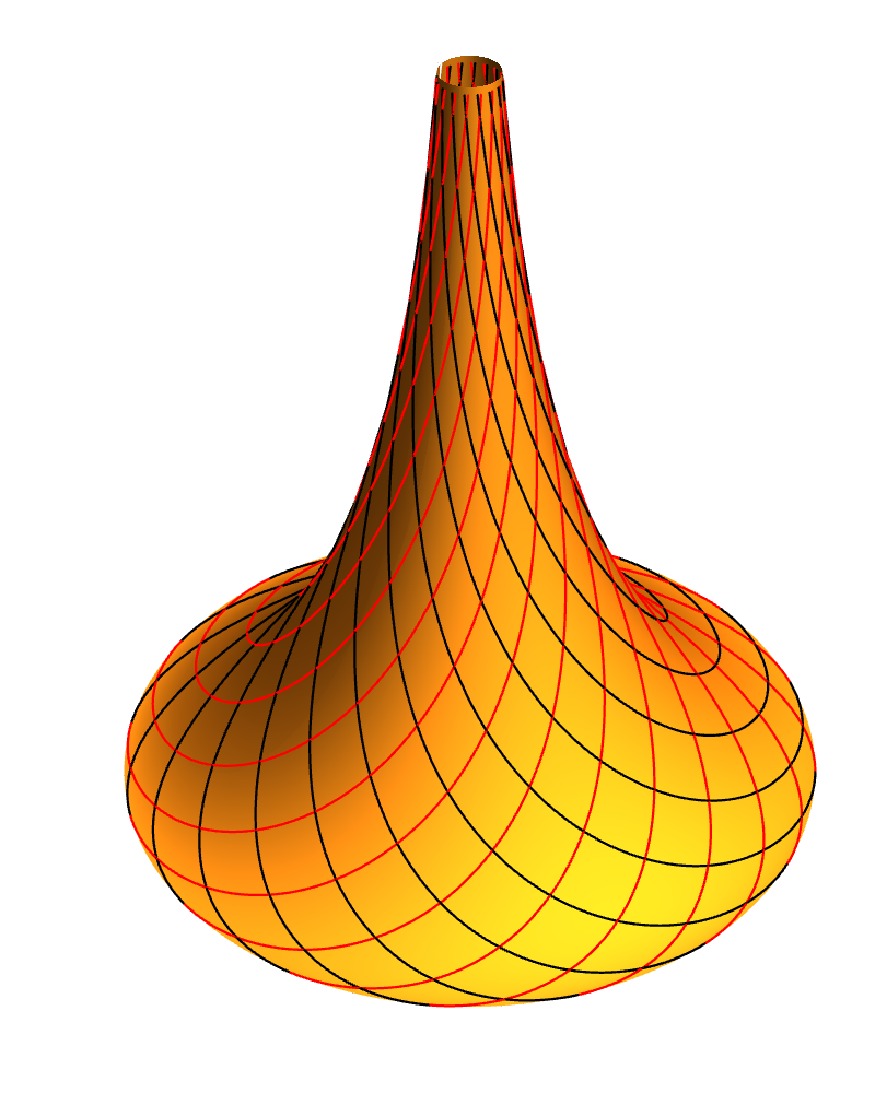 |
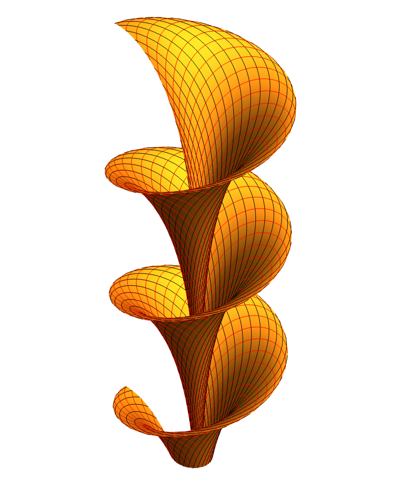 |
The metric here is just what we would expect, but the second fundamental form, S(u, v), tells us something new and interesting: the tangents to the u and v coordinate grid lines give directions in which the surface has zero curvature:
(1,0)T S(u, v) (1,0) = 0
(0,1)T S(u, v) (0,1) = 0
If we slice the surface at any point P with a plane that contains the normal to the surface and the tangent to either of these grid lines, the intersection of the plane with the surface will have a curvature of zero at P. Curves like these grid lines are known as asymptotic curves or asymptotic lines,[8] because their tangents point along the asymptotes of the hyperbolas that appear in plots of the kind shown at the start of the appendix, in the case of negative Gaussian curvature. The directions of maximum positive and negative curvature lie midway between the two asymptotes.
Any surface with negative Gaussian curvature will have two families of asymptotic curves, since at every interior point on the surface there must be two asymptotic directions, where the curvature of a normal section changes from positive to negative. Starting at any point, we can keep following one of these directions, integrating the vector field to trace out a curve.
The images on the right show parts of a tractroid, with a grid using the u, v coordinates derived above, and of Dini’s surface with the same kind of coordinates. Note that at the boundary, the metric in these coordinates becomes degenerate, with both grid lines pointing in the same direction.
For Dini’s surface, the parameterisation is:
x(u, v) = (√[1–b2] sech(U(u,v)) cos(u+v), √[1–b2] sech(U(u,v)) sin(u+v), √[1–b2] tanh(U(u,v)) – (u–v))
where U(u,v) = √[(1+b)/(1–b)] u – √[(1–b)/(1+b)] v
This parameterisation has the same properties as the u, v coordinates on the tractroid, and it is not a coincidence that the grid lines for a coordinate system where the metric has diagonal components of 1 are also asymptotic curves in both of these embeddings of the hyperbolic plane. But how can we show that these two properties will occur together more generally?
Suppose we have a surface embedded in three-dimensional space, with a coordinate system that gives it a metric with 1s on the diagonal:
g(u, v) =
xu · xu xu · xv xu · xv xv · xv =
1 cos(ω(u, v)) cos(ω(u, v)) 1
while the second fundamental form is:
S(u, v) =
xuu · n xuv · n xuv · n xvv · n =
L(u, v) M(u, v) M(u, v) N(u, v)
where the functions L(u, v), M(u, v), N(u, v) are yet to be determined.
By looking at the components of the metric and taking derivatives with respect to u and v, we obtain:
xu · xu = 1
xuu · xu = 0
xuv · xu = 0
xv · xv = 1
xuv · xv = 0
xvv · xv = 0
xu · xv = cos(ω(u, v))
xuu · xv = –sin(ω(u, v)) ∂uω(u, v)
xvv · xu = –sin(ω(u, v)) ∂vω(u, v)
From these dot products, and the definition of the second fundamental form’s components, we have:
xuu = (cos(ω(u, v)) xu – xv) ∂uω(u, v) / sin(ω(u, v)) + L(u, v) n
xvv = (cos(ω(u, v)) xv – xu) ∂vω(u, v) / sin(ω(u, v)) + N(u, v) n
xuv = M(u, v) n
Suppose we now calculate xuuv · n and xuvv · n. Starting from the equations above, in each case we have two different ways to perform the calculation that must agree, because the order in which we take partial derivatives makes no difference.
(∂v xuu) · n = (∂u xuv) · n
(cos(ω(u, v)) M(u, v) – N(u, v)) ∂uω(u, v) / sin(ω(u, v)) + ∂vL(u, v) = ∂uM(u, v)
(∂u xvv) · n = (∂v xuv) · n
(cos(ω(u, v)) M(u, v) – L(u, v)) ∂vω(u, v) / sin(ω(u, v)) + ∂uN(u, v) = ∂vM(u, v)
These two equations are known (in the general case, without specialising to the form of the metric we have imposed), as the Mainardi-Codazzi equations[9]. They must be satisfied by the components of the metric and the second fundamental form in order for them to be compatible, arising from the same surface.
A family of solutions that satisfies both these equations is:
L(u, v) = 0
N(u, v) = 0
M(u, v) = α sin(ω(u, v))
where α can take any value. But if we want the Gaussian curvature of the surface to be a constant, K, we must have:
K = det(S) / det(g) = –M(u, v)2 / sin(ω(u, v))2 = –α2
So the curvature must be negative, and for K = –1 we must have M(u, v) = ±sin(ω(u, v)). And we have already seen that ω(u, v) must satisfy the sine-Gordon equation.
We have not proved that there are no other solutions of the Mainardi-Codazzi equations, but this calculation shows that the two properties of the coordinate grid we noted in our example are compatible. This suggests that we ought to be able to find embeddings of the hyperbolic plane in three-dimensional space by the following strategy:
In order to perform the second step, one approach would be to find a way to construct the coordinate grid lines as curves in three-dimensional space. If we know the curvature, κ(s), and torsion, τ(s), of any curve as a function of its arc length parameter s, then the Frenet-Serret formulas let us construct the curve, up to an overall rotation and translation.
The magnitude of the curvature κ is the magnitude of the derivative of a unit-length tangent to the curve, with respect to arc length. Our coordinates u, v are already arc length parameters for the coordinate grid lines, so the curvatures in question are:
|κ1| = |xuu| = |(cos(ω(u, v)) xu – xv) ∂uω(u, v) / sin(ω(u, v))|
= |∂uω(u, v)|
|κ2| = |xvv| = |(cos(ω(u, v)) xv – xu) ∂vω(u, v) / sin(ω(u, v))|
= |∂vω(u, v)|
The magnitude of the torsion of a curve is the magnitude of the derivative of a unit normal to the plane spanned by the curve’s tangent and the tangent’s derivative, with respect to arc length. In our case, the unit normal to that plane is just the unit normal to the surface itself, since we have:
xu · n = xuu · n = 0
xv · n = xvv · n = 0
Taking the derivative with respect to each coordinate of the first zero dot product in each case:
∂u (xu · n) = 0
xuu · n + xu · ∂un = 0
xu · ∂un = 0
∂v (xu · n) = 0
xuv · n + xu · ∂vn = 0
xu · ∂vn = ±sin(ω(u, v))
∂u (xv · n) = 0
xuv · n + xv · ∂un = 0
xv · ∂un = ±sin(ω(u, v))
∂v (xv · n) = 0
xvv · n + xv · ∂vn = 0
xv · ∂vn = 0
Knowing these dot products, along with the fact that since n is a unit vector its derivatives are orthogonal to n itself, tells us enough about the derivatives to find the magnitude of the torsions:
∂un = ±(cos(ω(u, v)) xu – xv) / sin(ω(u, v))
|τ1| = |∂un| = 1
∂vn = ±(cos(ω(u, v)) xv – xu) / sin(ω(u, v))
|τ2| = |∂vn| = 1
(In fact the torsion of any asymptotic curve satisfies τ2 = –K, on any surface of negative curvature, regardless of whether or not K is constant.[10])
The sign of the torsion is chosen by convention to be positive for a right-handed helix and negative for a left-handed helix, and it turns out that we always have one family of asymptotic curves with each sign. When constructing our surface, we just have to give one family of curves positive torsion and the other negative torsion; if we swap the assignment, that will simply change the surface into its mirror image (which might or might not be a different shape than the original). The sign of the curvature depends on which direction along the curve we associate with an increase, rather than a decrease, of the coordinate value, so we can assign it arbitrarily.
We have already seen one exact solution of the sine-Gordon equation:
Solution of the sine-Gordon equation from the tractroid
ω(u, v) = acos(2 sech(u – v)2 – 1)
What about other surfaces of revolution with K = –1? If we find the asymptotic curves by integrating the unit-length vector fields that give a normal curvature of zero, we are led to the family of solutions:
Solutions of the sine-Gordon equation from surfaces of revolution
Parameter c < 1, c ≠ 0
ω(u, v) = acos(2 cd(√[c/(1–c)] (u – v), (c–1)/c)2 – 1)
Here cd is one of the twelve Jacobi elliptic functions.
A similar calculation for Dini’s surface yields:
Solutions of the sine-Gordon equation from Dini’s surface
Parameter –1 < b < 1
ω(u, v) = acos(2 sech(√[(1+b)/(1–b)] u – √[(1–b)/(1+b)] v)2 – 1)
For general surfaces of constant negative curvature built from helices:
Solutions of the sine-Gordon equation from surfaces built from helices
Parameters c < 1, c ≠ 0, –1 < b < 1
ω(u, v) = acos(2 cd(√[c/(1–c)] (√[(1+b)/(1–b)] u – √[(1–b)/(1+b)] v), (c–1)/c)2 – 1)
In going from the first two solutions to the third and fourth, we see an example of a method that can be used to get a whole family of new solutions to the sine-Gordon equation from any one solution. If ω(u, v) is a solution:
∂u,v ω(u, v) = sin(ω(u, v))
Define ω(α)(u, v) = ω(α u, v/α)
Then ∂u,v ω(α)(u, v)
= ∂u,v ω(α u, v/α)
= (α)(1/α) sin(ω(α u, v/α))
= sin(ω(α)(u, v))
The third of our surface-based solutions above can be obtained from the first, and the fourth from the second, by using this method with α = √[(1+b)/(1–b)].
This method is very simple as we have described it, but it is also worth noting that it arises from the relativistic invariance of the sine-Gordon equation, when viewed as a wave equation in one dimension of space and one of time! The sine-Gordon equation can be rewritten as:
∂t,t ω(x, t) – ∂x,x ω(x, t) + sin(ω(x, t)) = 0
where instead of the variables u, v we use x, t, with:
x = u + v
t = u – v
u = ½(x + t)
v = ½(x – t)
Here x and t are space-time coordinates, and the form of the equation is much closer to that of more familiar wave equations. If we apply a “boost” to our coordinate system, to change to the coordinates used by an observer with a speed of b times the speed of light as measured in the original coordinates, and then switch back to u, v coordinates, we get a new solution of the sine-Gordon equation, in precisely the way we did when changing from surfaces of revolution to surfaces generated by helices with parameter b. In fact, we could apply a boost directly in the u, v coordinates if we treat them as “null,” or light-ray, coordinates. You might recognise √[(1+b)/(1–b)] as the factor by which the frequency of light changes due to the Doppler shift, for an observer approaching a light source at a fraction of b times the speed of light, while its reciprocal √[(1–b)/(1+b)] is the corresponding factor for light coming from the opposite direction.
There is another method that lets us generate new solutions; this one, which is a bit more mysterious, is known as a Bäcklund transform. Suppose, as before, that we have an existing solution, ω(u, v). We then look for new solutions ω(β)(u, v) that satisfy the following equations:
Bäcklund transform for sine-Gordon equation
If ω(u, v) is an existing solution, then ω(β)(u, v) is a new family of solutions.
∂u ½(ω(β) – ω) = β sin(½(ω(β) + ω))
∂v ½(ω(β) + ω) = (1/β) sin(½(ω(β) – ω))
Differentiating the first equation with respect to v yields:
∂u, v ω(β) = ∂u, v ω + β cos(½(ω(β) + ω)) ∂v (ω(β) + ω)
= sin(ω) + 2 cos(½(ω(β) + ω)) sin(½(ω(β) – ω))
= sin(ω) + sin(ω(β)) – sin(ω)
= sin(ω(β))
The simplest solution we can start with is the trivial solution, ω = 0. The Bäcklund transform conditions are then:
∂u ω(β) = 2 β sin(½ω(β))
∂v ω(β) = (2 / β) sin(½ω(β))
We can make progress on this by treating ω(β) as an independent variable, and integrating the reciprocal of the common term in the derivatives above:
∫ (1 / sin(½ω(β))) dω(β) = 2 log(tan(ω(β)/4))
This suggests we look for solutions of the form:
ω(β) = ±4 arctan(exp(A u + B v))
which we can make into precisely what we need by setting A = β and B = 1/β:
Bäcklund transform of trivial solution ω = 0
Parameter β can take any non-zero value
ω(β) = ±4 arctan(exp(β u + v/β))
If we compute the cosine of this, it turns out to be:
cos(ω(β)) = 1 – 2 sech(β u + v/β)2
This is essentially the same as the solution we obtained from Dini’s surface, if we set β = √[(1+b)/(1–b)], and replace ω(u, v) with π – ω(u, –v).
This solution is often written in the arctan form, in space-time coordinates x, t, and with β = ±√[(1–V)/(1+V)], which gives us:
1-soliton solution of the sine-Gordon equation
Parameter –1 < V < 1
This is the solution from Dini’s surface, expressed in space-time coordinates.
ωV (x, t) = ±4 arctan(exp(±(x – V t) / √[1 – V2]))
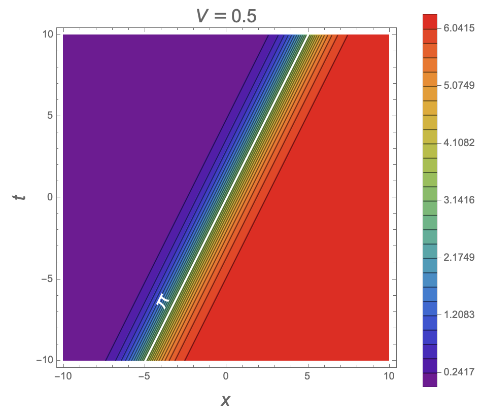
This is called the 1-soliton solution of the sine-Gordon equation, because it describes a travelling wave with a single fixed shape moving with a speed of V. Note that V can take on any value, positive or negative, with a magnitude less than 1; in the sine-Gordon equation, 1 corresponds to the speed of light. The value of ω goes from 0 for large negative values of ±(x – V t), to either 2π or –2π at large positive values. If we are thinking of ω as an angle, then 0, 2π and –2π are all the same, but ω either increases steadily across the whole wave, or decreases steadily, so it embodies a kind of twist.
When ω is an integer multiple of π, the two asymptotic curves of the associated surface become parallel, and the surface itself has a cusp where the curvature is undefined. So the line in the 1-soliton solution where ω = π corresponds to the boundary of Dini’s surface, and the whole x-t plane corresponds to two distinct copies of the surface. There is nothing to stop us gluing the two copies together along a shared boundary in three-dimensional space, but that will not give us a smooth isometry with a larger, single region of the hyperbolic plane.
Amazingly, it turns out that we can find solutions to the sine-Gordon equation from repeated applications of the Bäcklund transform without explicitly performing any further integrations. In 1892, the famous differential geometer Luigi Bianchi showed that Bäcklund transforms with different values of the parameter β commute, and this allowed him to construct the following solution:[11]
Bianchi solutions of the sine-Gordon equation
If ω is an existing solution, and ω(β1) and ω(β2) are derived from ω by single Bäcklund transforms,
then ω(β1, β2) is the result of two successive Bäcklund transforms.
ω(β1, β2) = ω + 4 arctan([(β2 + β1) / (β2 – β1)] tan(¼(ω(β2) – ω(β1))))
A direct computation, relying on ω being a solution of the sine-Gordon equation, and ω(β1) and ω(β2) being Bäcklund transforms of ω with parameters β1 and β2, confirms that ω(β1, β2) is a solution:
∂u,vω(β1, β2) – sin(ω(β1, β2)) = 0
We can iterate this process as many times as we wish. For example, suppose we pick three parameters, β1, β2, β3. The Bianchi solutions ω(β1, β2) and ω(β2, β3) correspond to applying Bäcklund transforms with the parameters β1 and β3 to the same initial solution ω(β2), so we can obtain a thrice-transformed solution:
ω(β1, β2, β3) = ω(β2) + 4 arctan([(β3 + β1) / (β3 – β1)] tan(¼(ω(β2, β3) – ω(β1, β2))))
The solutions we obtain by the Bianchi method that are reached by two Bäcklund transforms from the trivial solution are known as 2-soliton solutions. Some examples of these are given below, along with contour plots of the solution in space-time coordinates.
2-soliton KK collision
β1 = –√[(1–V)/(1+V)]
β2 = √[(1+V)/(1–V)]
Plus signs for amplitudes of both solutions
ωKK, V (x, t) = 4 arctan(V sinh(x / √[1–V2]) / cosh(V t / √[1–V2]))
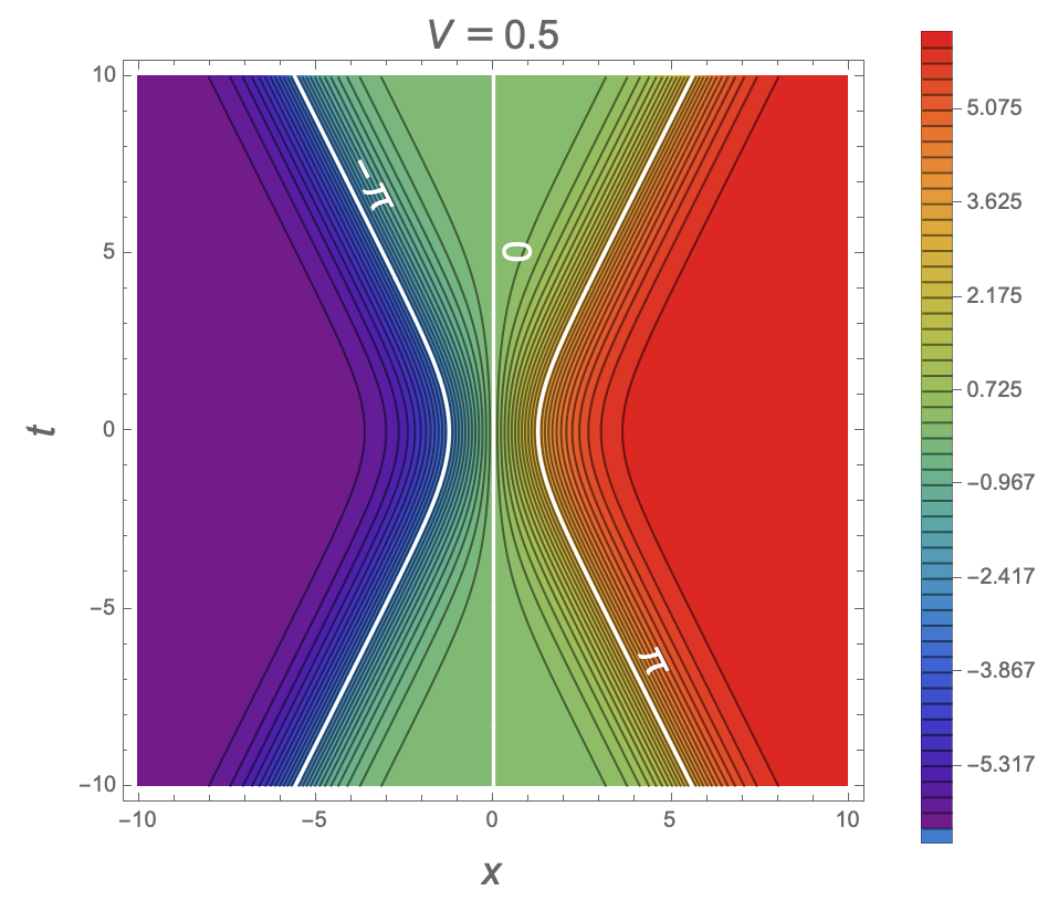
2-soliton KA collision
β1 = √[(1–V)/(1+V)]
β2 = –√[(1+V)/(1–V)]
Minus sign for amplitude of 1st solution, plus sign for 2nd solution
ωKA, V (x, t) = 4 arctan(V cosh(x / √[1–V2]) / sinh(V t / √[1–V2]))
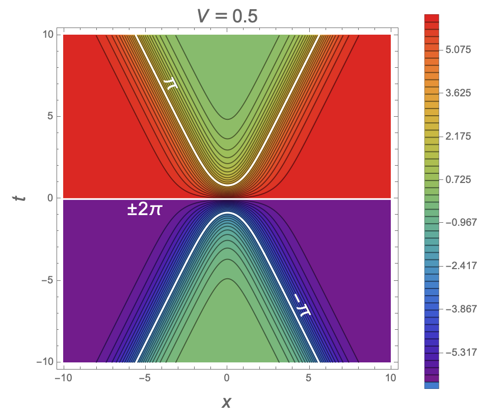
We can use complex values for β if they are complex conjugates of each other, resulting in real-valued periodic solutions known as “breathers.”[12]
Stationary “breather”
β1 = exp(i α)
β2 = exp(–i α)
Plus signs for amplitudes of both solutions
ωSB, α(x, t) = 4 arctan(cot(α) sin(sin(α) t) / cosh(cos(α) x))
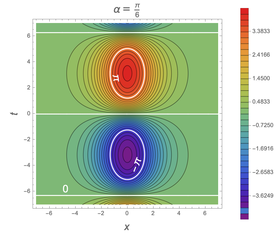
Bäcklund and Bianchi came across these transformations in the context of the following geometric problem. Suppose you have a surface S of constant negative curvature, and you try to construct a second such surface, Σ, by choosing a line segment at every point of S, tangent to S, of a fixed length, with its far end tracing out the new surface, Σ. By choosing the direction of the line segment at each point in the right way, can you make Σ into another surface of constant negative curvature?
The answer is yes! If the original surface is parameterised by x(u, v) with u, v measuring arc length along asymptotic curves, there is a family of new surfaces:[13]
New surface of constant curvature K = –1 via Bäcklund transform
ω is angle between asymptotic curves on original surface x(u, v).
ω(β), derived from ω by a Bäcklund transform, is angle between asymptotic curves on new surface x(β)(u, v).
x(β)(u, v) = x(u, v) + 2β / [(1+β2) sin ω(u, v)] (sin(½(ω(u, v) – ω(β)(u, v))) xu + sin(½(ω(u, v) + ω(β)(u, v))) xv)
On the new surface, the coordinates u, v again measure arc length along asymptotic curves.
In general, we will not have closed form expressions for geodesics on these surfaces, so to establish an isometry between such a surface and the hyperbolic plane, we can either find suitable geodesics on the surface by numerical methods, and identify them with known geodesics on the hyperbolic plane, or we can rely on the u, v coordinate grid on the surface, and use numerical methods to construct matching curves in the hyperbolic plane, with the same curvature and the same angles between them. We calculated the curvature, |κ1| and |κ2|, of the u, v curves previously, as curves in flat three-dimensional space, but for asymptotic curves this is the same as their geodesic curvature, which is measured relative to the geodesics of the surface.
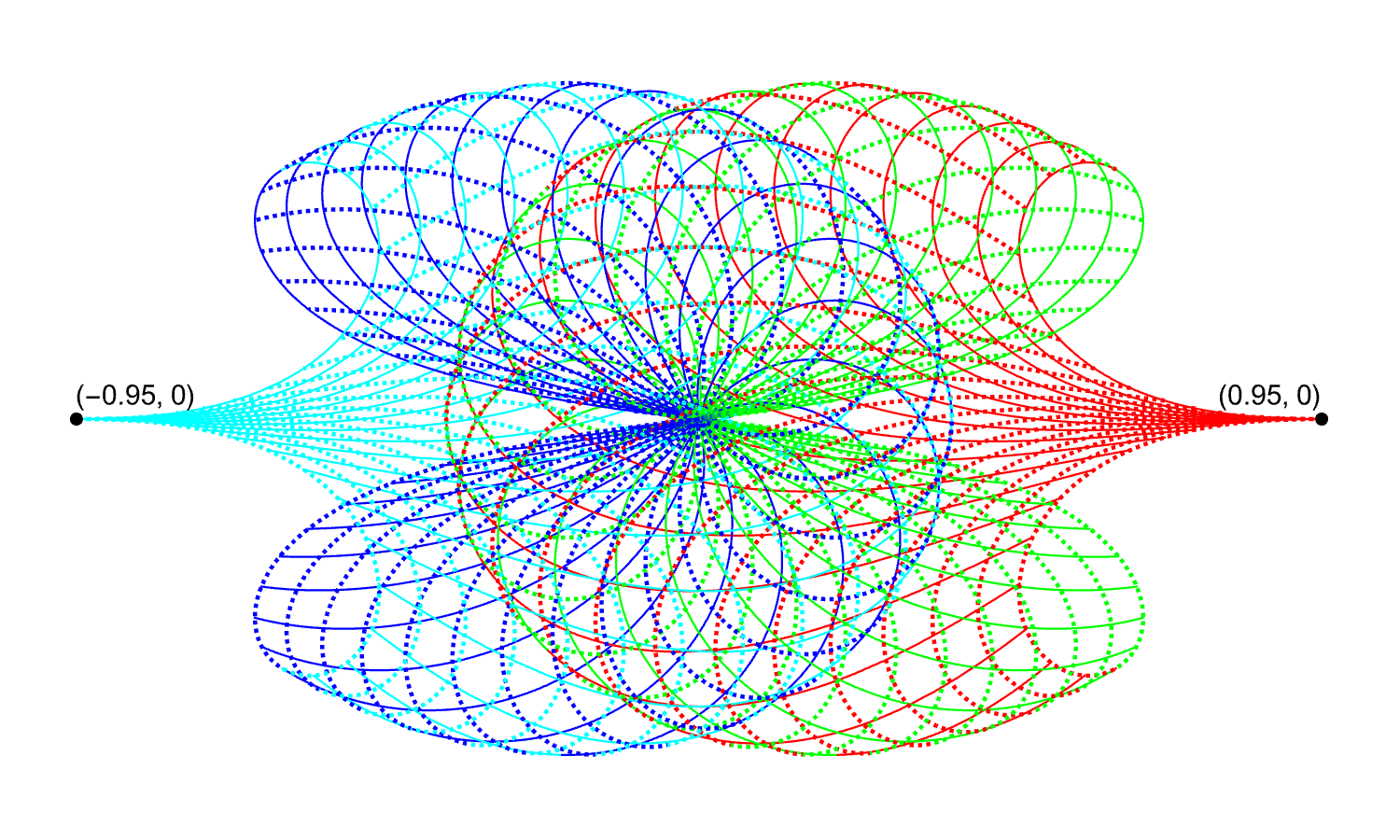
The image above shows the u, v coordinate grid that we obtain on the hyperbolic plane by matching the curvature of the grid lines to the 2-soliton KK solution for V = 0.5, with –π ≤ u, v ≤ π. (We are using the Poincaré disk model, but we have omitted the background tiling that we showed in previous images of the Poincaré disk, to avoid visual clutter.) The grid lines where u varies are solid, and those where v varies are dashed, and the different colours correspond to regions of the solution where ω lies between different integer multiples of π. As we cross the cusps where the u and v curves become parallel, ω crosses an integer multiple of π, and the grid wraps back onto the same region of the hyperbolic plane. So, this gives us four separate one-to-one isometries, mapping each of the four regions of the surface between these cusps to corresponding regions of four different copies of the hyperbolic plane.
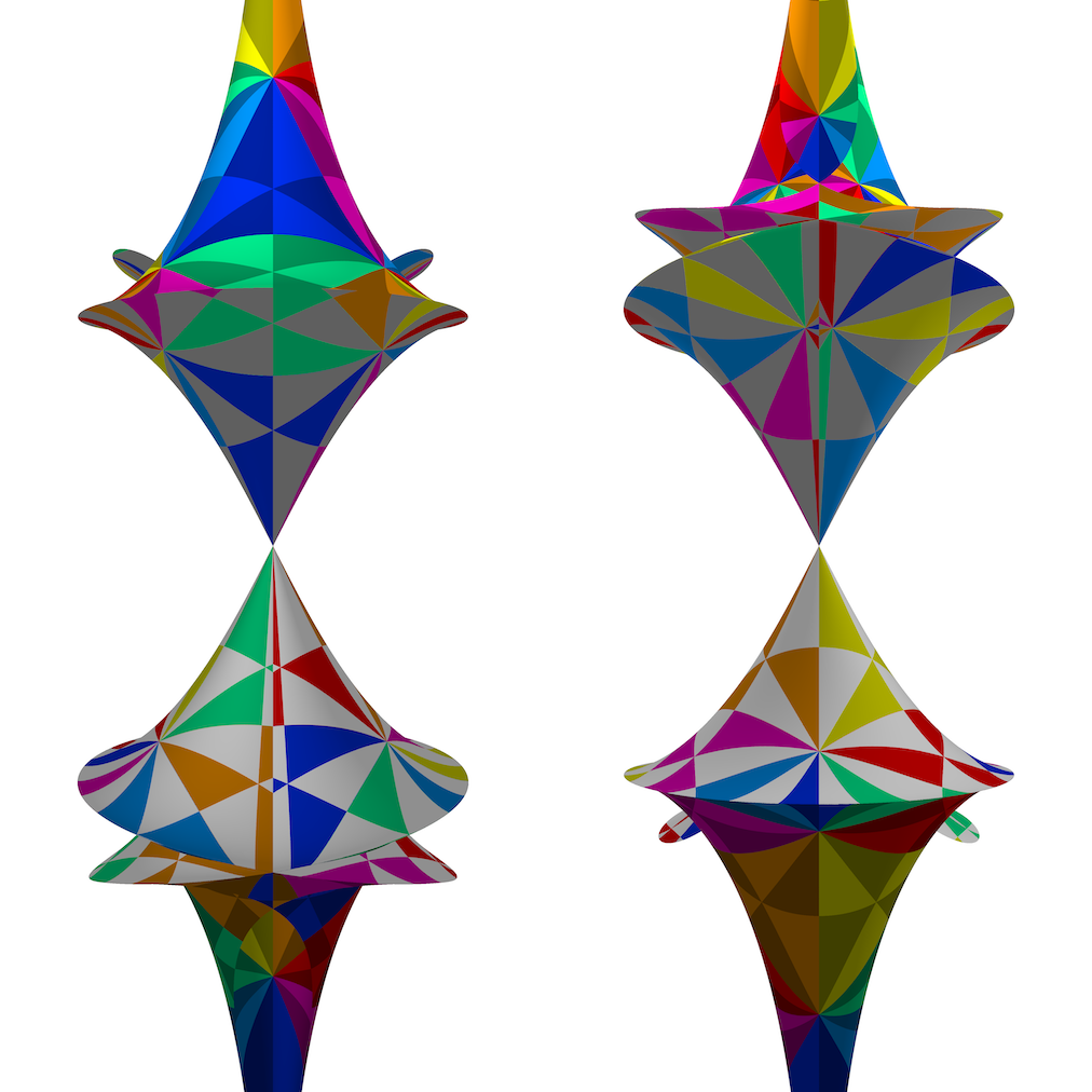 |
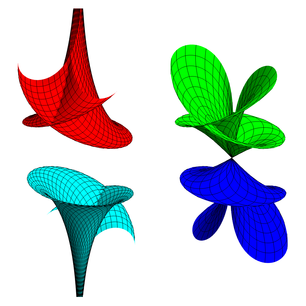 |
The image above left shows parts of the surfaces of constant negative curvature associated with the 2-soliton KK collision solution of the sine-Gordon equation, for values of the velocity parameter V cycling between 0.25 and 0.75, seen from two opposite viewpoints. For each surface, we have plotted the portion –π ≤ u, v ≤ π. There are four distinct regions separated by cusps corresponding to curves in the solution where ω is an integer multiple of π, and the different regions are indicated by changing the hues used in the tiling. The image above right shows the four individual regions, separated out into two pairs, for V = 0.5.
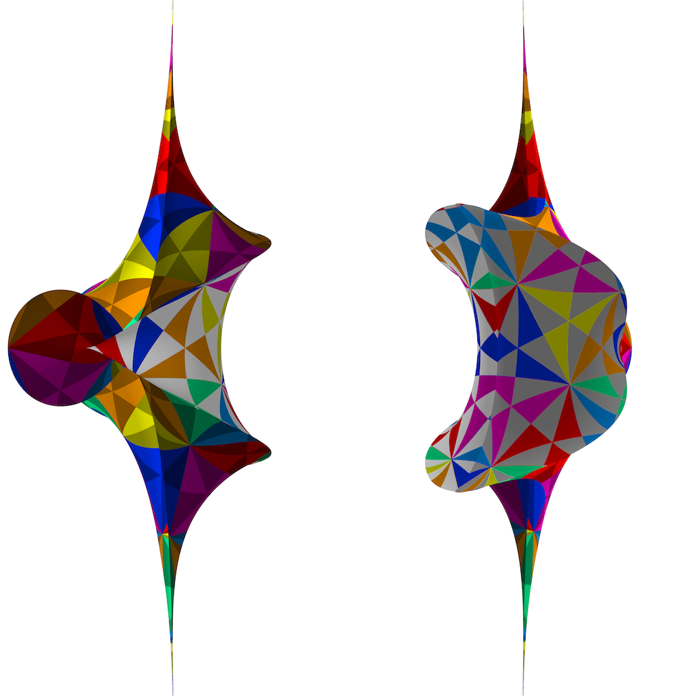 |
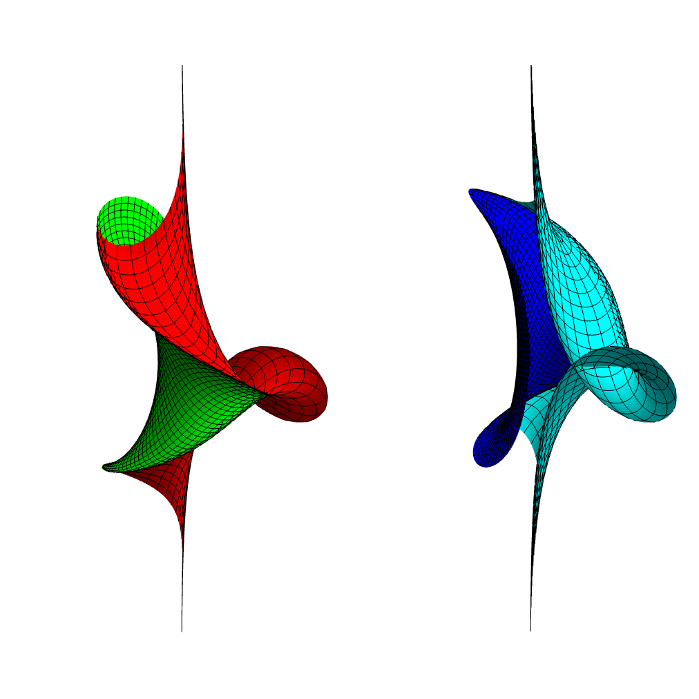 |
The image above left shows parts of the surfaces of constant negative curvature associated with the 2-soliton KA collision solution of the sine-Gordon equation, for values of the velocity parameter V cycling between 0.25 and 0.75, seen from two opposite viewpoints. For each surface, we have plotted the portion –π ≤ u, v ≤ π. As with the surface for the KK collision, there are four distinct regions separated by cusps corresponding to integer multiple of π, the different regions are indicated by changing the hues used in the tiling, and the image above right shows the individual regions for V = 0.5.
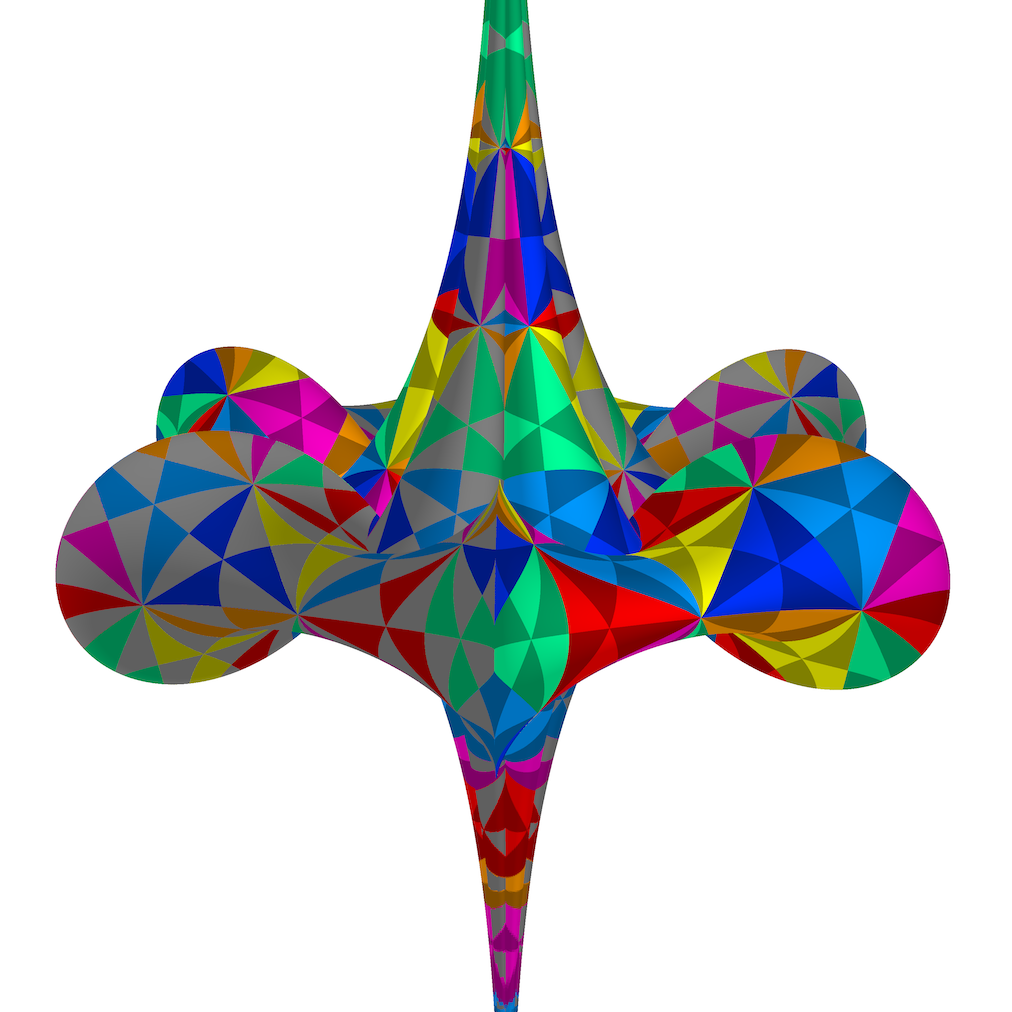 |
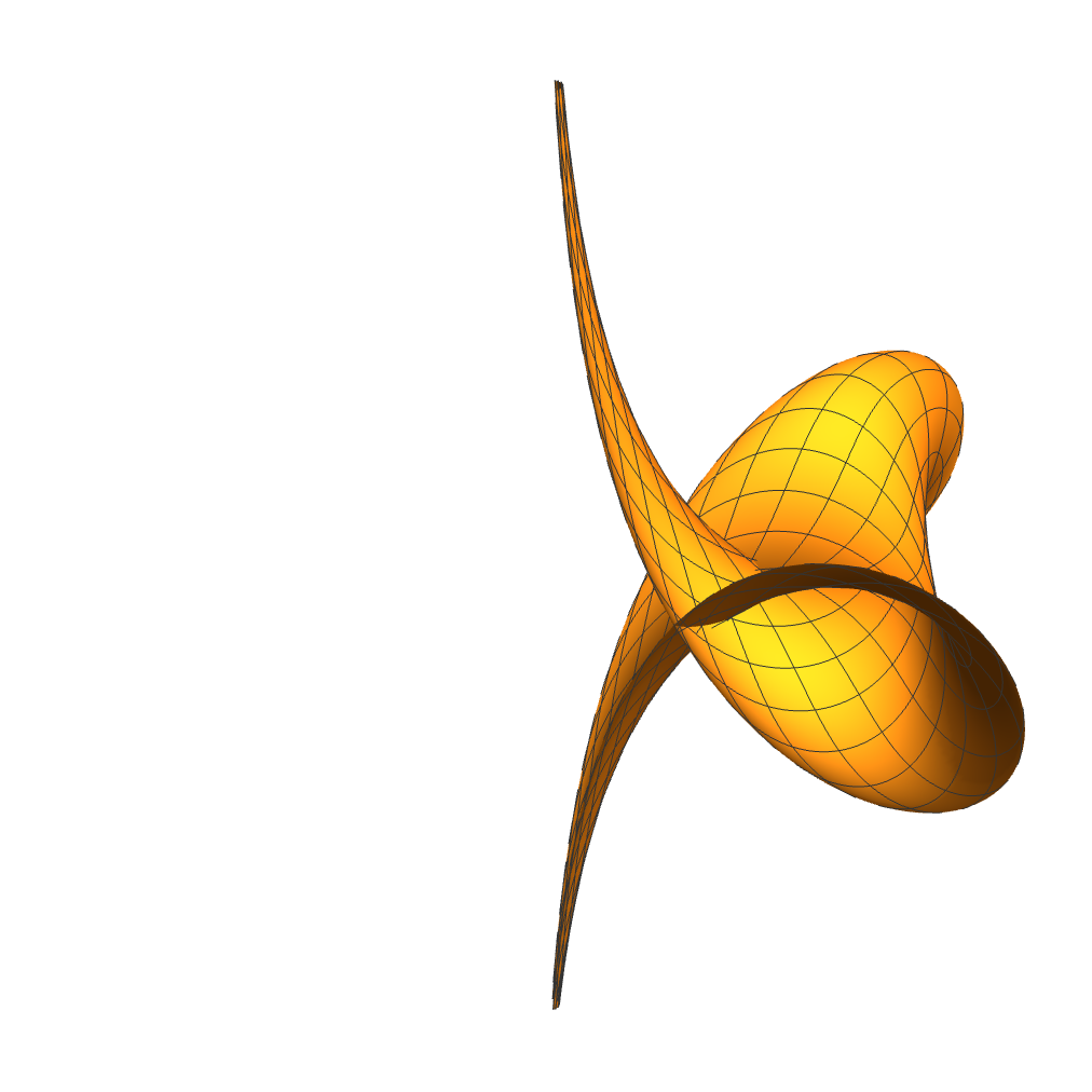 |
The image above left shows part of the surface associated with a stationary breather solution of the sine-Gordon equation, with sin(α) = 3/4; the image above right shows a single region between cusps. Choosing sin(α) = (q–1)/q will always produce a shape with 2(q–1)-fold symmetry like this.
Any rational value for sin(α) will generate a surface that closes up eventually. Suppose sin(α) = p/q, where p and q are integers and we have cancelled any common factors. Then it can be shown that the angle around the axis between successive cusps is given by:
Δφ = (1/sin(α) – 1) π = (q – p)/p π
For p = q – 1 we have Δφ = π/(q – 1), which divides 2π, but in general Δφ will only divide some multiple of 2π.
Note that:
p Δφ = π (q – p)
2 p Δφ = 2 π (q – p)
are both integer multiples of π, and the first will be an integer multiple of 2π if and only if q – p is even. So the surface will close up after wrapping around the axis q – p times if q – p is odd, and ½(q – p) times if it is even.
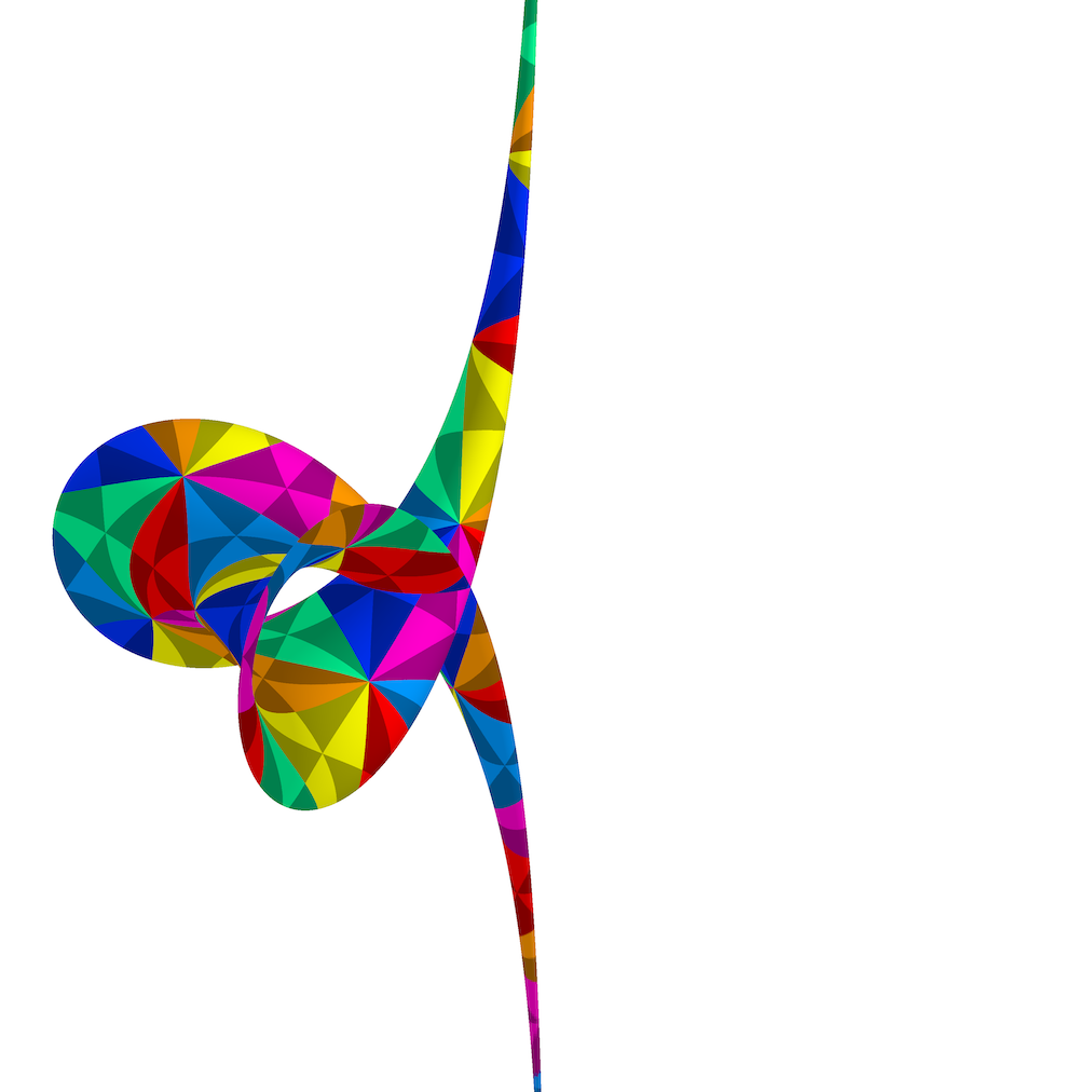 |
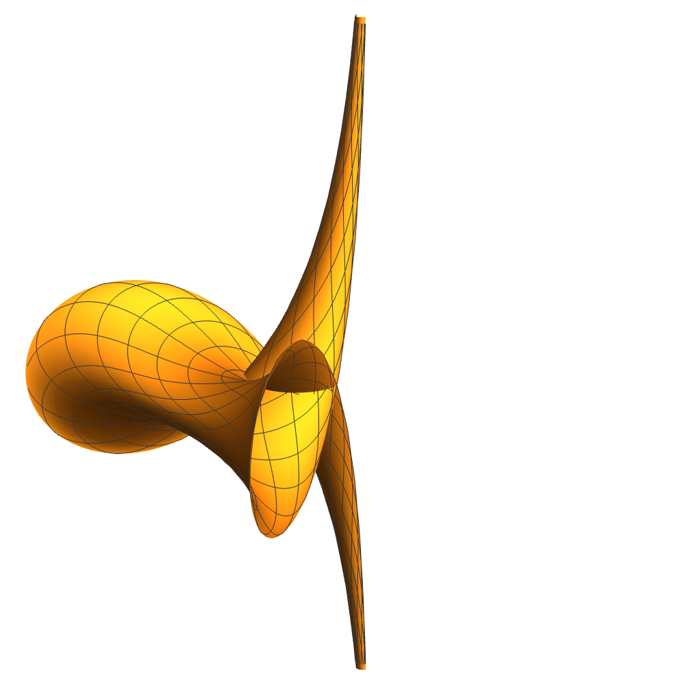 |
The images above show a single cusp-to-cusp portion of the surface associated with a stationary breather, as sin(α) ranges between 3/4 and 1/3.
For sin(α) = 1/3 we have Δφ = 2π, so the surface wraps completely around the axis.
When α falls below π/4, the breather solution reaches values that cross ±π, which introduces a new cusp inside each portion of the surface. These cusps correspond to the roughly elliptical white contours that can be seen in the second plot in the breather solutions shown earlier.
Earlier, we showed that given any smooth, non-self-intersecting curve c(s) in three-dimensional Euclidean space, there is an intrinsically flat surface that contains this curve, and for which this curve is a geodesic. Intuitively, what we are doing is taking a strip of paper and positioning a straight line drawn on it to coincide with the three-dimensional curve c(s).
Can we do the same thing for surfaces with constant non-zero Gaussian curvature? The intrinsically flat surface we found was generated by a family of lines, and I am not aware of an equally simple construction for K ≠ 0, but we can set up a system of partial differential equations whose solution will give us the surface we want.
For our purposes, it will be convenient to choose a coordinate system for the surface where u corresponds to longitude on a sphere and v corresponds to latitude (measuring both in radians), or analogous coordinates on the hyperbolic plane. The curve where u varies and v is fixed at zero, the “equator,” will be a geodesic. The curves where v varies and u is fixed (at any value) will correspond to meridians, i.e. geodesics that meet the equator orthogonally. The curves where u varies and v is fixed at a non-zero value will correspond to circles of latitude, which are not geodesics. A simple calculation shows that the geodesic curvature of a circle of lattitude on a sphere is κg = √|K| tan v, while the corresponding curve on the hyperbolic plane (i.e. a curve that lies at a fixed distance v/√|K| from some geodesic) has κg = √|K| tanh v.
We know the components of the metric in these coordinates, and we can write both cases in a similar form:
For K > 0, define s(v) = sin v, c(v) = cos v
For K < 0, define s(v) = sinh v, c(v) = cosh v
xu · xu = c(v)2 / |K|
xv · xv = 1 / |K|
xu · xv = 0
Differentiating each of these three equations with respect to u and v, we obtain:
xu · xuu = 0
xu · xuv = –c(v) s(v) / K
xv · xuv = 0
xv · xvv = 0
xv · xuu = –xu · xuv = c(v) s(v) / K
xu · xvv = –xv · xuv = 0
These dot products are enough to let us write xu in terms of derivatives that are purely with respect to v, or xv in terms of derivatives that are purely with respect to u.
PDEs for surface of constant Gaussian curvature K
For K > 0, define s(v) = sin v, c(v) = cos v
For K < 0, define s(v) = sinh v, c(v) = cosh v
If supplied curve x(0, v) is like a meridian, from which we generate curves of varying u like circles of latitude:
xu = ±c(v) / |xvv| (xvv × xv)
If supplied curve x(u, 0) is like the equator, from which we generate curves of varying v like meridians:
xv = c(v) s(v) / [K |xuu|2] xuu ± √[1 – c(v)2 s(v)2 / (|K| |xuu|2)] / (|xuu| c(v)) (xuu × xu)
The first equation will apply if we wish to treat our initial curve as a “meridian” with fixed longitude u and varying latitude v, which we then extend by computing the curves of varying u, corresponding to circles of latitude. The second equation will apply if we treat the initial curve as the “equator” with v = 0 and varying longitude u, which we then extend by computing the geodesics of varying v, corresponding to meridians.
The quantity:
c(v) s(v) / (|xuu| √|K|)
shows up, squared, inside the square root in the second PDE. This can be understood geometrically as the ratio between the geodesic curvature of a circle of latitude:
κg = √|K| s(v) / c(v)
and its curvature as a space curve:
κ = |K| |xuu| / c(v)2
When the absolute value of the ratio, |κg/κ|, exceeds 1, it becomes impossible for the curve to be embedded in a surface in such a way that it has the correct geodesic curvature. At this point, the quantity inside the square root in the second PDE becomes negative, making it clear that the integration cannot continue, and we have reached the edge of the surface. It’s easy to check that this is what happens at the endpoints of the meridians of the surfaces of revolution we examined earlier, if we choose u to be the angular coordinate, and the curves of constant v, as space curves, are all just circles. For example, for the hourglass-like surfaces of constant negative curvature, described by a parameter ξ that is greater than 1, the length (measured from the waist) of the meridians is:
L = a arctanh(1/ξ)
and at the boundary, the radius of the circles of latitude is:
ρmax = a ξ
So at the boundary, we have:
κg = √|K| sinh(v) / cosh(v)
= tanh(v) / a
= tanh(L / a) / a
= 1 / (a ξ)
κ = 1 / ρmax = 1 / (a ξ)
However, it is also possible for |κg/κ| to be less than 1 while the extrinsic curvature of the surface goes to infinity, also marking a boundary.
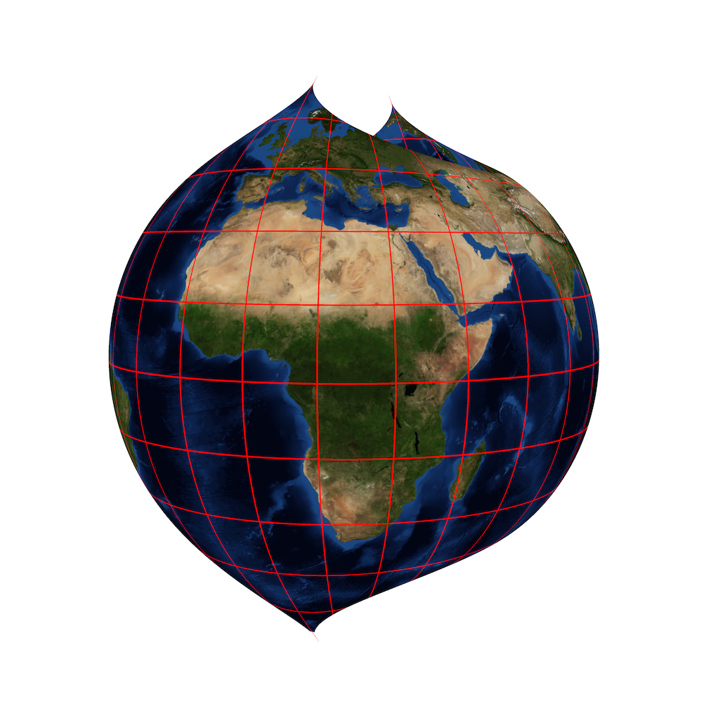 |
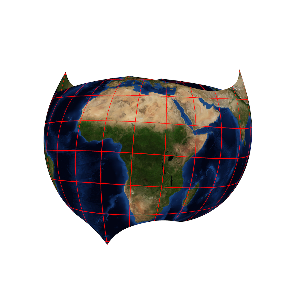 |
The image above left shows a family of surfaces of constant positive Gaussian curvature that contain an ellipse as a geodesic. The length-to-width ratio of the ellipse ranges from 1.05 to 1.5, but the overall scale is adjusted to keep the perimeter constant at 2π, the same as the equator of a unit sphere. In effect, these surfaces are the maximal portions of an idealised world globe, made of a material that can be bent but not stretched or sheared, that allow the equator to be deformed into the ellipses in question. As the aspect ratio of the ellipse becomes more extreme, the surface encompasses less of the original globe, with the range of latitude shrinking most along the meridians where the curvature of the equator is reduced the most, i.e. in the region where the ellipse is narrowest.
The image above right shows a similar family of surfaces where the curve chosen for the geodesic corresponding to the equator is non-planar:
(r cos t, r sin t, h cos 2t)
with the ratio h/r ranging from 0.05 to 0.5, while again the overall scale is adjusted to keep the total length of the curve equal to 2π. So these surfaces correspond to the maximal portions of an idealised globe that allow the equator to be deformed into this non-planar curve.
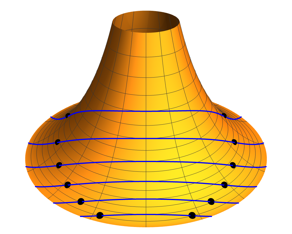 |
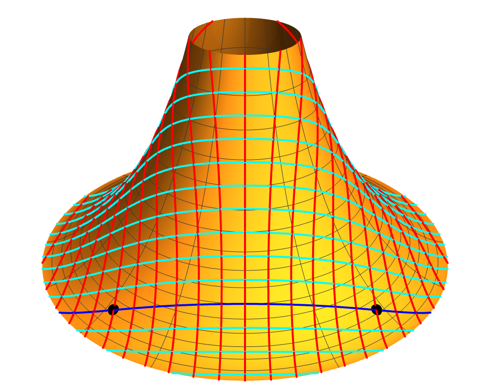 |
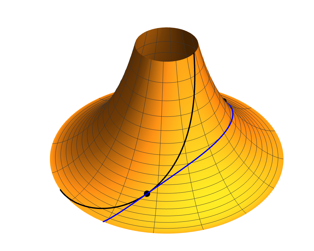 |
The partial differential equations for surfaces of constant curvature containing a specified curve as a geodesic need to be treated carefully when the curve contains inflection points, i.e. points where its curvature as a space curve is zero, since the quantity |xvv| or |xuu|, which appears in the denominator of terms in these equations, goes to zero at such points. Of course the equations can still make sense if the numerators also go to zero sufficiently rapidly, so the ratio can be interpreted as a finite limit as the inflection point. But we can say a couple of things independently of the equations, just by thinking about the geometry.
First, no surface with positive Gaussian curvature everywhere can contain a smooth curve with an inflection point. This follows from the fact that the normal curvature (as discussed in the appendix) must range between two positive values as we rotate the plane normal to the surface, with which we slice it to produce the normal sections. The curvature of these normal sections is equal to the length of the projection, onto the normal to the surface, of the curvature vector of any curve passing through the same point in the same direction,[14] and so a curve with zero curvature would allow for zero normal curvature, which is impossible.
For a surface with negative Gaussian curvature, the situation is very different. A hyperboloid can contain straight lines, as we have seen, and Dini’s surface contains a single straight line, the z-axis, that is a geodesic. Every non-meridian geodesic on the tractroid (such as the blue lines in the image on the top right) contains two points of inflection (marked in black). So, if the curve we nominate to be a geodesic for a surface of constant negative curvature contains inflection points, that need not be an obstacle to the surface existing in some finite region around those points.
Let’s look at that last example a bit more closely. For the tractroid with a = 1, along geodesics of the form:
ρ(s) = ρ0 cosh(s), where s ranges from –arccosh(1/ ρ0) to arccosh(1/ ρ0)
φ(s) = tanh(s)/ρ0
(x, y, z) = (ρ cos(φ), ρ sin(φ), arccosh(1/ρ) – √[1 – ρ2])
the squared curvature of the geodesic as a space curve is:
κ(s)2 = (1 – ρ02 cosh(s)4)2 / [ρ02 cosh(s)6 (1 – ρ02 cosh(s)2)]
So there are inflection points at:
s = ±arccosh(1/√ρ0)
(where ρ = √ρ0
and φ = ±√[1 – ρ0]/ρ0)
Any geodesic like this will be intersected orthogonally at any given value of s by another geodesic (red curves in the image on the middle right), with parameter t:
ρs(t) = ρ0 sinh(s) cosh(t), where t ranges from –arccosh(1/ [ρ0 sinh(s)]) to arccosh(1/ [ρ0 sinh(s)])
φs(t) = [tanh(t)/sinh(s) + coth(s)] / ρ0
The two geodesics intersect orthogonally at:
t = –arccosh(coth(s))
cosh(t) = coth(s)
tanh(t) = sinh(s) tanh(s) – cosh(s)
If we set s = u and t = v – arccosh(coth(u)), this puts a new set of coordinates on the tractroid, with the properties discussed at the start of this section, and which satisfy the partial differential equation that we derived for xv. In the image on the middle right, the blue curve is the original geodesic v = 0 [the “equator”], the cyan curves are non-geodesic curves of constant v [“circles of latitude”], and the red curves are geodesics of constant u [“meridians”].
We have seen that an inflection point in a curve need not be an obstacle to that curve being a geodesic of a surface of constant negative Gaussia curvature. However, there are further restrictions that we need to consider.
If a geodesic has an inflection point, i.e. a point of zero curvature, then its tangent must be pointing in one of the asymptotic directions[8] of the surface at that point: a direction such that all curves have a normal curvature of zero. So, the geodesic will share its tangent with an asymptotic curve (the black curve in the image on the bottom right).
The asymptotic curve at this point has its curvature vector orthogonal to the normal to the surface, whereas the geodesic, though it has a zero curvature vector at the point itself, has a principal normal vector (the unit vector parallel or antiparallel to the curvature vector, extended by continuity across inflection points) that is parallel or antiparallel to the normal to the surface. So, the instantaneous planes in which the two curves lie are momentarily locked together, at a right angle to each other. This means the torsion, the rate at which those planes rotate, must be the same (or opposite) at this point.
But we saw earlier that the torsion of any asymptotic curve on a surface of constant Gaussian curvature of –1 is τ = ±1, and more generally τ2 = –K.[10] So, in order for a curve with an inflection point to be a geodesic of a surface of constant Gaussian curvature K, its torsion at that point must satisfy the same equation (or the inflection point must be of a different kind, with not only the curvature, but also its derivative, being zero).
Another way to see this is to explicitly calculate two of the three independent components of the second fundamental form along the supplied curve, in the case where we treat that curve as an “equator”, and assuming K = –1.
On the equator, v = 0, we have:
n = ±xuu / |xuu|
xuu · n = ±|xuu|
= ±κ(u), the curvature of x(u, 0)
xv = xu × xuu / |xuu|
xuv = ∂u xv
= xu × xuuu / |xuu| – [(xuuu · xuu) / |xuu|3] xu × xuu
xuv · n = ± ((xu × xuuu) · xuu) / |xuu|2
= ±τ(u), the torsion of x(u, 0)
This is enough to let us write the second fundamental form, on the equator, as:
S(u, 0) =
xuu · n xuv · n xuv · n xvv · n =
±κ(u) ±τ(u) ±τ(u) ∓(1 – τ(u)2) / κ(u)
Here, we have filled in the lower right corner of the matrix by the requirement that K = det(S) / det(g) = –1, and the fact that det(g) = 1 in our chosen coordinates. This shows us that the torsion τ(u) must be ±1 at any point where the curvature κ(u) is zero, in order for the lower right entry of the second fundamental form to have a finite limit (assuming that the derivative of κ(u) there is non-zero).
But this restriction on the torsion of the curve at the inflection points is still not enough to guarantee that we can construct a surface of constant negative curvature. If we compute the third derivative, xvvv, it contains terms that, near the inflection point u0, include factors of the form:
[κ'(u0) τ''(u0) – κ''(u0) τ''(u0)] / (u – u0)
The numerator here must vanish in order for the v-curve through the inflection point to have a finite third derivative. This amounts to the requirement that the curvature and torsion have series expansions:
κ(u0 + ε) = κ1 ε + κ2 ε2 + ...
τ(u0 + ε) = ±1 + α (κ1 ε + κ2 ε2) + ...
for some constant α. This is not hard to arrange. But for higher derivatives, there are further, increasingly complex conditions that must be met.
How can we construct a curve that meets this infinite set of restrictions at an inflection point? Obviously the tractroid geodesics that we discussed earlier, and any other geodesic with an inflection point that we find on a known surface of constant negative curvature, will meet all the conditions, but we want to be able to construct new surfaces, not just reconstruct known cases.
One approach would be to start by specifying a curve, M, that has a torsion of ±1 but a non-zero curvature at some point P, treating it as a “meridian”, and using the first of our PDEs to construct a surface whose “equator” E meets M at P. The curve E will then have an inflection point at P. This follows from the same calculations we used to construct the second fundamental form, where the lower right entry can now be seen as the curvature of M at P, and the condition on the determinant becomes:
det(S) = ±κM(P) κE(P) – τM(P)2 = –1
Since τM(P) = ±1 and κM(P) ≠ 0, this can only be satisfied by κE(P) = 0, so E must have an inflection point at P.
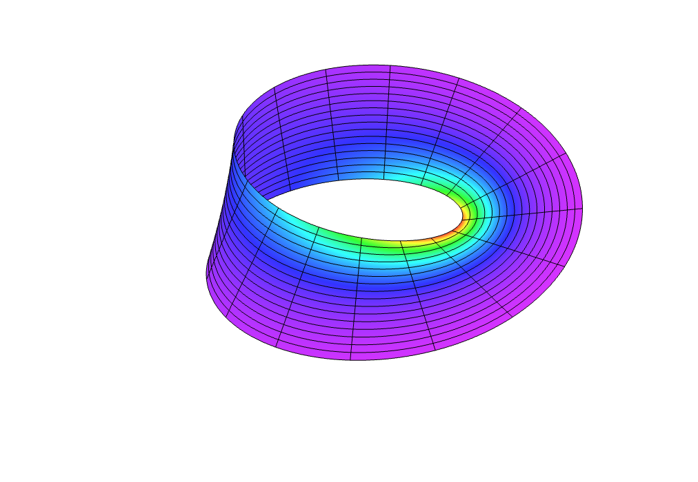
The simplest way to construct a Möbius strip is to choose a circle as the centreline, then sweep out a surface by taking a line segment orthogonal to the circle at some point and move it around the circle, while rotating it by half the angle through which it has moved. As it comes back to its starting point, it will have been rotated by 180 degrees, putting the required twist into the surface. If the circle has radius R, and the coordinates on the surface are θ for the angle around the circle and s for the distance along the line segment, the surface has Cartesian coordinates:
x(θ, s) = (R + s cos(½θ)) cos(θ)
y(θ, s) = (R + s cos(½θ)) sin(θ)
z(θ, s) = s sin(½θ)
The image on the right shows a Möbius strip like this. The surface has been coloured according to its Gaussian curvature at each point, with red for the most negative curvature, shading to purple for values closer to zero, but still negative. So this surface is not flat, but nor does it have a constant negative curvature. And the centreline here is not a geodesic, because the curvature vector for the circle always points radially inwards, which is generally not a direction normal to the surface.
Now, suppose we want to construct a Möbius strip whose surface has a constant Gaussian curvature of K = –1, and whose centreline is a geodesic of the surface.
We previously showed how to construct a Möbius strip that was intrinsically flat, with its centreline as a geodesic. It would be nice if we could take the same centreline:
(x(t), y(t), z(t)) = (3 sin(t), cos(t) + (2/5) cos(2t) + (1/15) cos(3t), (3/4) sin(2t))
and apply one of our partial differential equations for surfaces of constant Gaussian curvature to extend it into a surface with K = –1. Unfortunately, this is impossible! This centreline contains an inflection point (a point where the curvature, κ, is zero) at t = π, and it was one of the requirements of the construction that the torsion, τ, must go to zero at any such point at least as rapidly as the curvature. But as we saw in the previous section, the torsion at any inflection point on a geodesic of a surface of constant Gaussian curvature K must satisfy τ2 = –K.
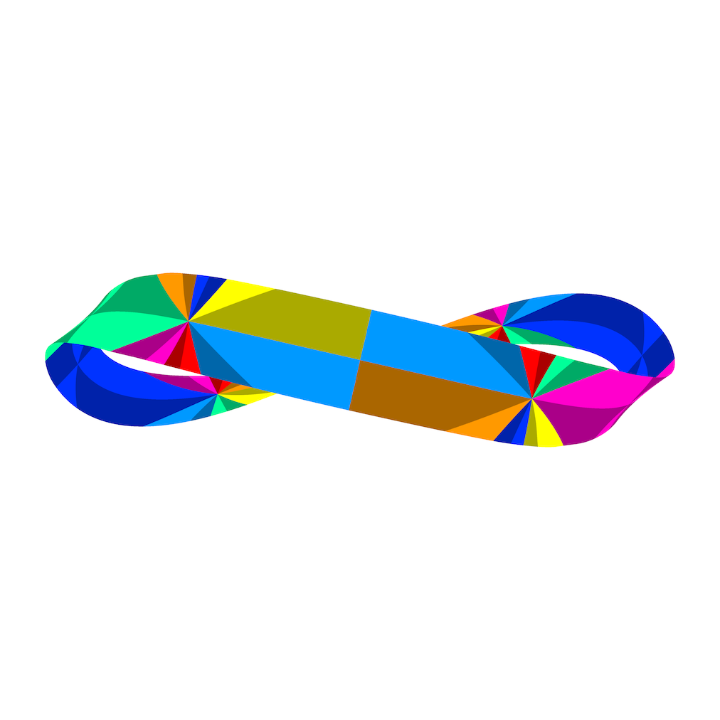
And as we also discussed in that section, there are actually an infinite number of conditions that must be satisfied at the inflection point in order for all the derivatives of the orthogonal coordinate curve to be finite. These conditions are increasingly complex, and I am not aware of any way to reframe them as a single equation the original curve could satisfy that would guarantee they were all met. Alternatively, if we tried to work backwards by specifying an orthogonal curve with finite derivatives and a torsion of 1, we would obtain a candidate centreline curve with an inflection point, but there would be no easy way to guarantee that it formed a loop.
In lieu of any perfect solution, we can construct a curve numerically that meets the conditions required for some chosen number of derivatives of the orthogonal coordinate curve to be finite. The surface itself can then be approximated with a Taylor series in each of the three Cartesian coordinates.
The image on the right has a centreline that is a sum of trigonometric functions:
x(t) = sin(t)
y(t) = 0.715336 cos(t) – 0.222511 cos(2t) + 0.0194119 cos(3t) + 0.000532444 sin(2t)
z(t) = 0.145095 sin(2t) + 0.00409208 sin(3t) – 0.0094447 sin(4t) + 0.00238777 sin(5t) – 0.00024958 sin(6t)
These coefficients have been chosen to produce an inflection point at t = 0, and also to meet the conditions required for the sixth-order Taylor series for the orthogonal coordinate curves to have finite derivatives everywhere on the centreline.
The idea of combining spatial dimensions and time into a single mathematical structure known as spacetime is the central insight of special relativity. [This does not mean simply adding a fourth dimension to three-dimensional Euclidean space and then treating it identically to all the rest. For a sketch of how the distinction between the space and time dimensions works mathematically, try this simple overview, which I wrote as part of the background to a series of novels set in an alternative universe in which the distinction is absent, and all four dimensions are spacelike.]
The spacetime equivalent of flat Euclidean space is known as Minkowski spacetime, and though this term usually refers to three space dimensions and one of time, the same general idea works with any total dimension. Minkowski spacetime with two spatial dimensions and one of time is fairly easy to visualise with three-dimensional spacetime diagrams, so long as we remember that the actual geometry (the lengths, times and angles) can be different from what we see.
In Minkowski spacetime, the version of Pythagoras’s theorem that applies to flat Euclidean space is replaced with one where, rather than just adding up the squares of all the perpendicular distances between two points in order to find the square of the straight-line distance between them, we subtract the square of the time difference between points in the spacetime. For example, for the simple case of computing the squared distance from the origin (0, 0, 0) of a point with coordinates (t, x, y) in Minkowski spacetime with two spacelike dimensions and one of time, we have (in units where the speed of light equals one):
squared distance from origin of (t, x, y) = –t2 + x2 + y2
This “distance” is sometimes referred to by the more formal term the spacetime interval. If t is large enough, it can be zero or negative. When the squared spacetime interval is positive, negative, or zero, the vector (t, x, y) is described, respectively, as spacelike, timelike, or null. The term lightlike is also used as a synonym for null.
Nearby points along the world line of a material object are separated by timelike vectors; more precisely, the tangent to such a world line is timelike. This amounts to saying that material objects are always found to be travelling slower than light. Similarly, the tangents to the world lines of photons are null vectors. No physical object has a world line with a spacelike tangent; spacelike separations between events indicate that you would need to move faster than light to travel between them.
For a two-dimensional surface where both dimensions are spatial, a single number at each point, the Gaussian curvature, describes the intrinsic curvature of the surface. The same is true for a two-dimensional surface where one dimension behaves like space and the other like time. In this case, the number used is generally the Ricci scalar curvature, which can be computed for any number of dimensions and any metric signature (that is, any number of the dimensions being timelike as opposed to spacelike). For ordinary two-dimensional surfaces, the Ricci scalar curvature is exactly twice the Gaussian curvature.
If we take Minkowski spacetime with two dimensions of space and one of time and embed a surface within it, the surface will inherit a geometry from the ambient Minkowski spacetime. We can measure the type (spacelike, timelike or null) and magnitude of any vector within the surface by making the same measurement in the Minkowski spacetime. This is just the spacetime equivalent of what we did when embedding surfaces in three-dimensional Euclidean space.
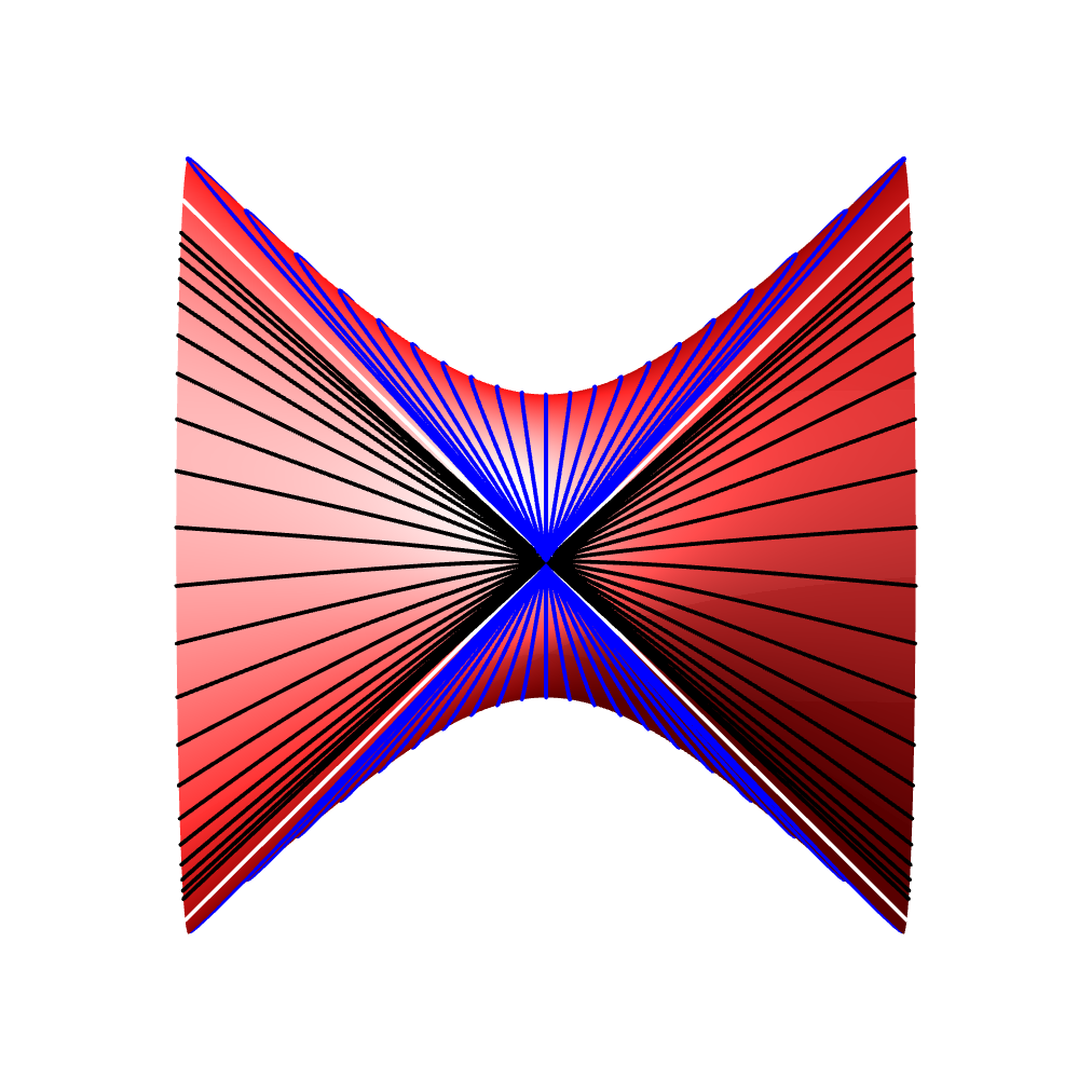
In the image on the right, the red hyperboloid is a surface whose spacetime interval measured from the origin has a constant spacelike value of a, which means it is described by the equation:
–t2 + x2 + y2 = a2
The time axis, the axis of symmetry of the hyperboloid, is drawn horizontally here. We have truncated the hyperboloid in the diagram at a finite distance along the axis, but mathematically it continues to infinity along the time axis in both directions. If we wish, we can also consider the surface to be infinite in the direction that wraps around the axis, by supposing that we switch to a new portion of the surface every time we come full circle.
This surface is known in mathematics and cosmology as a two-dimensional de Sitter spacetime. It has a constant Ricci scalar curvature of 2/a2, which is the same as that of a sphere of radius a in three-dimensional Euclidean space (that is, twice the Gaussian curvature of 1/a2).
The image includes a set of geodesics that all pass through one point. The black curves are timelike geodesics, the blue curves are spacelike geodesics, and the white curves are null geodesics.
Note that the blue spacelike geodesics move apart but then come together again on the opposite side of the hyperboloid, just like the great circles through any point on a sphere. In contrast, the black timelike geodesics continue to move apart.
We won’t go into the formal definition of the Ricci scalar curvature, but the behaviour of the spacelike geodesics already suggests a useful intuitive definition, by analogy with the behaviour of the geodesics on a sphere and its connection with the Gaussian curvature. On a sphere, if you take two nearby geodesics and call the distance between them D(s), where s is the distance along the geodesics from some arbitrary starting point to the point where you measure the distance between them, then in the limit of “infinitesimally close” geodesics it turns out that the second rate of change of the geodesic separation is given by:
d2 D(s) / ds2 = –K D(s)
where K is the Gaussian curvature of the sphere.
To verify this, consider two meridians on a sphere of radius a, separated by a small difference in longitude, say δ. If we set s = 0 where the meridians cross the equator, the latitude of the points on both of them where we measure their separation D(s) will be s/a, and so the radius of the circle of latitude containing those points will be R(s) = a cos(s/a). For small δ, we then have:
D(s) = R(s) δ
= δ a cos(s/a)
d2 D(s) / ds2 = –(δ/a) cos(s/a)
= –(1/a2) D(s)
= –K D(s)
What we will show is that the second rate of change of the separation between geodesics in our two-dimensional de Sitter spacetime obeys the same kind of relationship, where the equivalent of K is 1/a2 for spacelike geodesics, –1/a2 for timelike geodesics, and 0 for null geodesics.
We will start by describing the de Sitter hyperboloid in terms of coordinates T and X on the surface, with (T, X) corresponding to the point in Minkowski spacetime:
H(T, X) = (t, x, y) = (a sinh T, a cosh T cos X, a cosh T sin X)
We then have:
–t2 + x2 + y2
= a2 (–sinh2 T + cosh2 T (cos2 X + sin2 X))
= a2 (–sinh2 T + cosh2 T)
= a2
as required. The coordinate vectors on the surface correspond to vectors in Minkowski spacetime:
HT = (a cosh T, a sinh T cos X, a sinh T sin X)
HX = (0, –a cosh T sin X, a cosh T cos X)
The metric for the de Sitter spacetime with these coordinates is given by:
g(T, X) =
HT · HT HT · HX HT · HX HX · HX =
–a2 0 0 a2 cosh2 T
where the dot product we have used comes from the Minkowski spacetime, so it has a minus sign for the time component:
(t1, x1, y1) · (t2, x2, y2) = –t1 t2 + x1 x2 + y1 y2
The rotational symmetry of the hyperboloid means that adding any constant θ to the X coordinates on the surface maps it into itself isometrically, by rotating the hyperboloid by an angle θ. We can use Killing’s theorem, as we have previously, to find a simple characterisation of the geodesics on the surface that follows from this symmetry. For a geodesic with coordinates:
G(λ) = (TG(λ), XG(λ))
and tangent:
∂G/∂λ = (∂TG/∂λ, ∂XG/∂λ)
we have, from Killing’s theorem and the symmetry under uniform changes in X, a quantity C that is invariant along that geodesic:
(∂G/∂λ)T g(G(λ)) (0,1) = C
(∂XG/∂λ) a2 cosh2 TG = C
One family of solutions for spacelike geodesics is given by:
Spacelike geodesics in de Sitter spacetime.
λ is distance along geodesic from X = 0.
T0 is T coordinate at λ = 0.
TG(T0, λ) = asinh[cos(λ/a) sinh T0]
XG(T0, λ) = atan[tan(λ/a) / cosh T0]
Define χ = cosh TG = √[1 + cos(λ/a)2 sinh2 T0]
Derivatives:
∂TG/∂λ = –sin(λ/a) sinh T0 / [a χ]
∂XG/∂λ = cosh T0 / [a χ2]
∂TG/∂T0 = cos(λ/a) cosh T0 / χ
∂XG/∂T0 = –sin(λ/a) cos(λ/a) sinh T0 / χ2
Invariant along geodesic:
(∂XG/∂λ) a2 cosh2 TG = a cosh T0
This family of geodesics have G(0) = (T0, 0), and ∂G/∂λ at λ = 0 is (0, 1/[a cosh T0]), so they will all pass orthogonally through the meridian X = 0 on the hyperboloid. After a distance of a π/2 they will then converge on a single point:
G(a π/2) = (0, π/2)
So these are the geodesics we have already seen as the blue curves on the diagram shown previously.
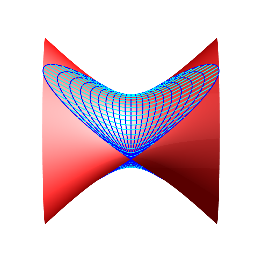
What is the second rate of change of the distance between two nearby geodesics in this family?
The image on the right shows the family of spacelike geodesics in blue, along with (non-geodesic) curves that mark an equal distance along all the geodesics in the family (cyan). Each cyan curve can be thought of as parameterised by T0 along its length, for a different fixed value of λ.
From the derivatives of the T and X components given above, we find that the blue and cyan curves are perpendicular wherever they cross, and ∂G/∂T0, the tangent to the cyan curves, is a timelike vector with magnitude:
|∂G/∂T0| = a cos(λ/a)
The magnitude of this vector is essentially the “distance between nearby geodesics,” because the vector is perpendicular to the geodesics, and its magnitude measures the distance between them, per unit change in T0, in the limit as that change, δ, goes to zero. So we have:
D(λ) = δ a cos(λ/a)
d2 D(λ) / dλ2 = –(1/a2) D(λ)
This show that the spacelike geodesics here converge just as they do on a sphere.
This family of geodesics includes all the spacelike geodesics that pass through one of its points of convergence. To see this, we can compute the tangent at λ = a π/2:
∂G/∂λ | λ = a π/2 = (–(sinh T0)/a, (cosh T0)/a)
Since T = 0 at this point, the metric is just a2 times the 1+1 (one space, one time) Minkowski metric, and by a choice of T0 (and multiplying by ±1) these tangents give us all the unit spacelike vectors.
One simple family of timelike geodesics that are initially parallel and then diverge is:
Timelike geodesics in de Sitter spacetime.
λ is time along geodesic from T = 0.
X0 is X coordinate on the entire geodesic.
TG(X0, λ) = λ/a
XG(X0, λ) = X0
Derivatives:
∂TG/∂λ = 1/a
∂XG/∂λ = 0
∂TG/∂X0 = 0
∂XG/∂X0 = 1
Invariant along geodesic:
(∂XG/∂λ) a2 cosh2 TG = 0
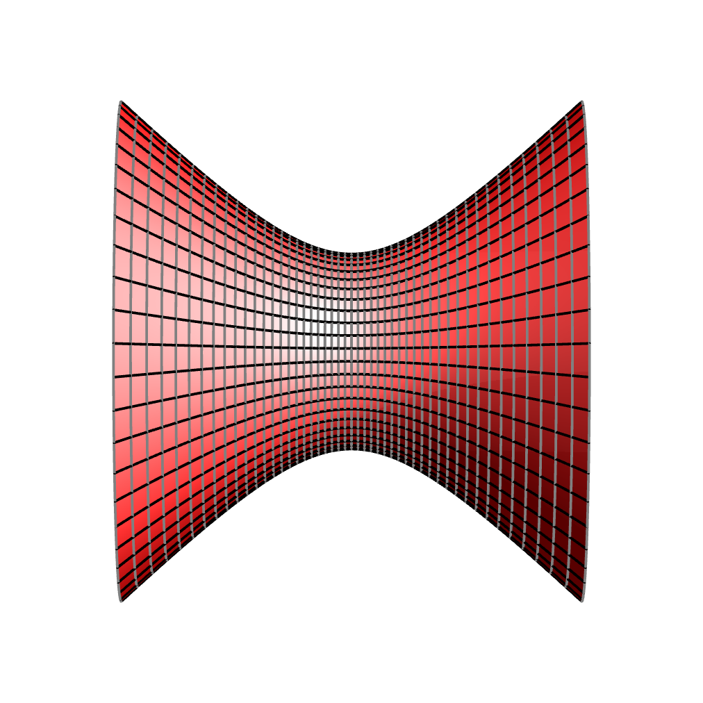
In the image on the right the black curves are the timelike geodesics, and the grey curves mark equal times along those geodesics. The two kinds of curve are perpendicular when they cross.
In this case, the tangent to the grey curves, ∂G/∂X0 is a spacelike vector with magnitude:
|∂G/∂X0| = a cosh(λ/a)
and the divergence of the geodesics shows up in the sign of the second derivative as:
D(λ) = δ a cosh(λ/a)
d2 D(λ) / dλ2 = (1/a2) D(λ)
Unlike the family of spacelike geodesics, this family clearly does not give us all the timelike geodesics through a point, so for completeness we will mention another family that does:
Timelike geodesics in de Sitter spacetime.
λ is time along geodesic from the point T = 0, X = 0.
μ is parameter for tangent at λ = 0.
TG(μ, λ) = asinh[sinh(λ/a) cosh μ]
XG(μ, λ) = atan[tanh(λ/a) sinh μ]
Define χ = cosh TG = √[1 + sinh(λ/a)2 cosh2 μ]
Derivatives:
∂TG/∂λ = cosh(λ/a) cosh μ / [a χ]
∂XG/∂λ = sinh μ / [a χ2]
∂TG/∂μ = sinh(λ/a) sinh μ / χ
∂XG/∂μ = sinh(λ/a) cosh(λ/a) cosh μ / χ2
Invariant along geodesic:
(∂XG/∂λ) a2 cosh2 TG = a sinh μ
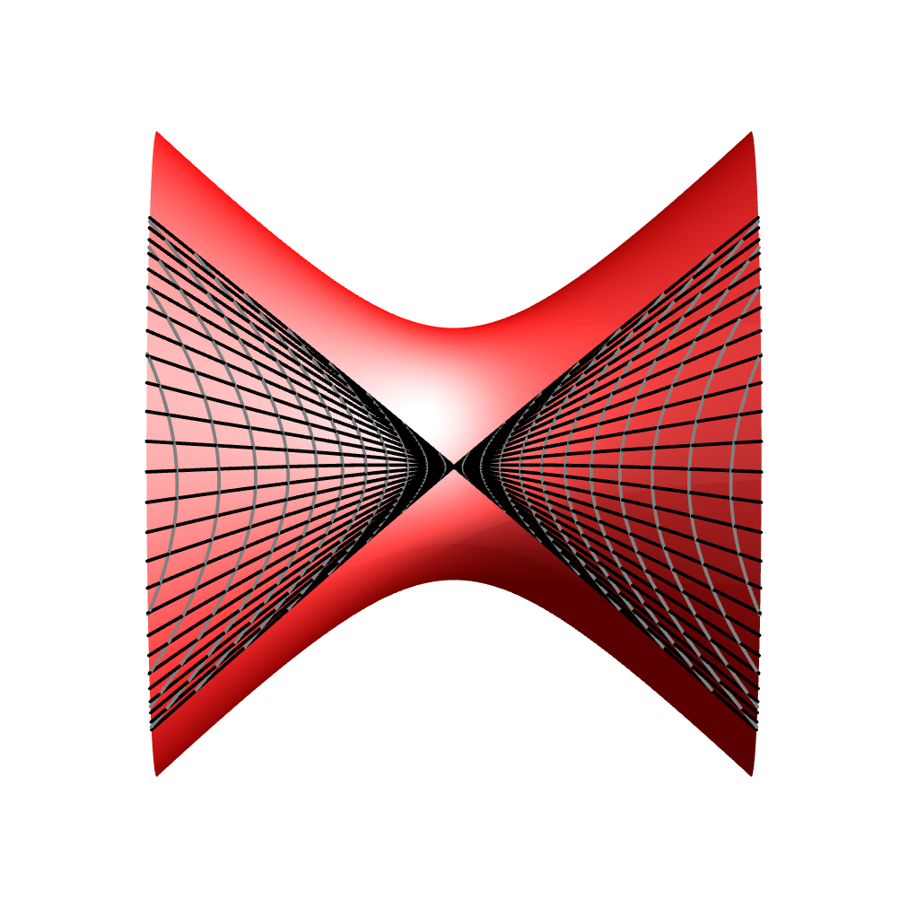
In the image on the right, the black curves are the timelike geodesics, and the grey curves mark equal times along those geodesics. Once again, the two kinds of curve are perpendicular when they cross.
At λ = 0 these geodesics all pass through T = 0, X = 0, where their tangent can take on any timelike unit vector with a positive T component, as specified by the parameter μ.
The separation between geodesics in this family can be tracked by seeing that the tangent to the grey curves, ∂G/∂μ, is a spacelike vector with magnitude:
|∂G/∂μ| = a sinh(λ/a)
Nearby geodesics in this family are never parallel (that is, the derivative with respect to λ of their separation is never zero). But for the second derivative, the separation satisfies the same differential equation as the simpler family of timelike geodesics:
D(λ) = δ a sinh(λ/a)
d2 D(λ) / dλ2 = (1/a2) D(λ)
Here is a family of null geodesics:
Null geodesics in de Sitter spacetime.
λ is affine parameter along geodesic from T = 0.
X0 is X coordinate at λ = 0.
TG(X0, λ) = asinh[λ/a]
XG(X0, λ) = X0 + atan[λ/a]
Define χ = cosh TG = √[1 + (λ/a)2]
Derivatives:
∂TG/∂λ = 1 / [a χ]
∂XG/∂λ = 1 / [a χ2]
∂TG/∂X0 = 0
dXG/X0 = 1
Invariant along geodesic:
(∂XG/∂λ) a2 cosh2 TG = a
We parameterised the spacelike geodesics by the length measured along the curve, and the timelike geodesics by the time, but for null geodesics the spacetime interval measured along the curve is zero. So how can we choose an appropriate parameter?
The key to this is the notion of parallel transport, which is a way of taking a vector at one point in a curved space or spacetime, and carrying it along a path in a way that keeps it “as parallel as possible” to its initial direction. In general, two vectors at different points in a curved space or spacetime cannot be compared, but with parallel transport we can still guarantee some useful properties of the transported vectors:
The tangent to a geodesic G(λ) is the derivative of its coordinates with respect to the parameter, ∂G(λ)/∂λ. There is a special class of parameters, the affine parameters, such that the tangent to the geodesic satisfies the following condition:
If we parallel transport the tangent vector to a geodesic at some point A along that geodesic to another point B, the transported tangent from A agrees with the locally computed tangent at B.
In the context of a space or spacetime with a suitable symmetry, the tangent to the geodesic must also give an invariant quantity as required by Killing’s theorem. And in the specific case of null geodesics on the rotationally symmetric, two-dimensional surface of the hyperboloid, that the tangent vector is a null vector, and that its dot product with the Killing vector is constant, are enough to show that the choice of λ for our family of null geodesics is an affine parameter.
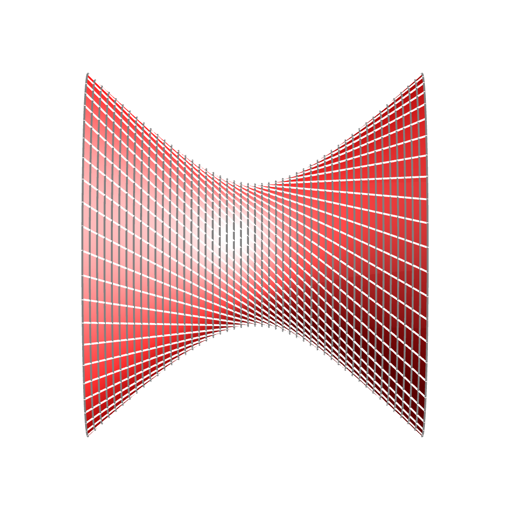
In the image on the right, the white curves are the null geodesics, and the grey curves mark equal values of the affine parameter λ along those geodesics. However, the two kinds of curve are not perpendicular when they cross.
We claimed earlier that the second derivative of the separation between null geodesics is zero, from which it would follow that nearby null geodesics travelling in the same direction have a constant separation. However, there are some subtleties in making this precise. For the timelike and spacelike geodesics, we could measure their separation in a direction perpendicular to their tangent, but for a null vector in two dimensions only multiples of the vector itself have a dot product with it of zero, so a perpendicular vector will never take us from one null geodesic to another.
In fact, there is no well-defined, coordinate-independent notion of “the true separation” between two null geodesics in a two-dimensional spacetime. For our family of null geodesics, if we use |∂G/∂X0| to measure the separation — ignoring the fact that this vector is not perpendicular to the geodesics — we find that:
|∂G/∂X0| = √[a2 + λ2] = a cosh T
This corresponds to the expanding radius of the circles of constant λ as we move away from λ = T = 0, but it is an arbitrary, coordinate-dependent choice. It might seem to make sense if we compare it with the cosmological red shift, where the distance between successive wavefronts of a light wave increases with the expansion of the universe, but that depends on singling out a particular set of observers, at rest with respect to the galaxies around them. In a completely empty spacetime, there is no preferred choice like that.
For the solution to this problem, we need to turn again to the notion of parallel transport. For the families of spacelike and timelike geodesics, when we measured their separation along directions perpendicular to the geodesics we could have equally well stated that the vector we were using to make the measurement was a unit-length vector, initially perpendicular to the geodesic, that we parallel-transported along the geodesic.
For a null geodesic, we cannot impose the condition that the measurement vector is perpendicular to it, but we can still insist that it should be parallel-transported. Our mistake, then, is that a unit-length vector in the direction of ∂G/∂X0 as we defined it is not parallel-transported. We can be sure of this, because if we divide ∂G/∂X0 = (0,1) by its magnitude to get a unit vector u, the dot product of u with the tangent to the geodesic will not be constant.
Since the curves of constant λ do not meet our requirements, we can look to assign a new parameter, say μ, along each geodesic, such that the curves of constant μ, still parameterised by X0, have tangents with respect to X0 that are parallel-transported along each null geodesic. There is no need for μ to be an affine parameter for the null geodesics, as we can continue to use λ to compute the tangents to the geodesics.
Suppose the relationship between the two parameters is given by:
λ = F(X0, μ)
The tangent to the curves of constant μ is then given by:
∂G/∂X0 | const μ = (∂F/∂X0 / √[a2 + F2], 1 + a ∂F/∂X0 / [a2 + F2])
The dot product of this with the tangent to the geodesics is:
(∂G/∂X0 | const μ)T g(G(X0, μ)) (∂G/∂λ) = a
so this is constant regardless of our choice of F. The squared magnitude of the tangent to the curves of constant μ is:
(∂G/∂X0 | const μ)T g(G(X0, μ)) (∂G/∂X0 | const μ) = a2 + F2 + 2 a ∂F/∂X0
We need this to be constant along each null geodesic:
∂ (a2 + F2 + 2 a ∂F/∂X0) / ∂μ = 0
2 F (∂F/μ) + 2 a ∂2F/(∂X0 ∂μ) = 0
F (∂F/μ) = –a ∂2F/(∂X0 ∂μ)
One family of solutions to this partial differential equation is:
F(X0, μ) = 2 a α tanh(α X0 + β μ + γ)
where α, β, γ are free parameters. It is straightforward to verify that this solves the equation:
∂F/μ = 2 a α β sech(α X0 + β μ + γ)2
∂2F/(∂X0 ∂μ) = –4 a α2 β sech(α X0 + β μ + γ)2 tanh(α X0 + β μ + γ)
= F (∂F/μ) / (–a)
Because the function tanh can only take values between –1 and 1, for a given choice of α we can only cover a finite portion of the geodesics. But since we can reach every part of every geodesic with some choice of α, the existence of these solutions still implies that all the null geodesics are at a “constant separation” everywhere, according to our definition: the vectors δ ∂G/∂X0 | const μ, which join pairs of null geodesics separated by an infinitesimal change δ in X0, have constant magnitude. And we can compute the value of the squared magnitude:
(∂G/∂X0 | const μ)T g(G(X0, μ)) (∂G/∂X0 | const μ)
= a2 + F2 + 2 a ∂F/∂X0
= a2 + 4 a2 α2 tanh(α X0 + β μ + γ)2 + 4 a2 α2 sech(α X0 + β μ + γ)2
= a2 (1 + 4 α2)
Of course this actual value has no meaning. But the fact that it is constant for any specific choice of α means that we can join two infinitesimally close null geodesics with a vector, and then if we parallel transport that vector along the geodesics the transported vector will continue to join them.
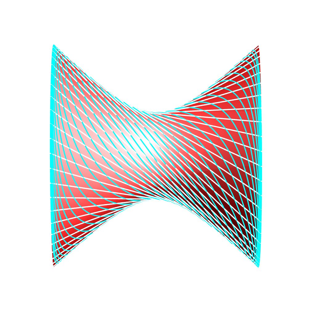
The image on the left shows an example of the curves (cyan), whose tangents with respect to X0 have the properties required to demonstrate that the null geodesics (white) have “constant separation”.
We assume that the surfaces we’re dealing with are described by mathematical functions whose second derivatives exist, and are continuous, everywhere, except perhaps along their boundaries. So at any interior point P on the surface we can always approximate its shape in a small region using a Taylor series. If we choose the origin of our coordinates to lie on the point P, and choose the z-axis to be orthogonal to the surface, the Taylor series up to quadratic terms in x and y can be written in the form:
z(x, y) = ½ A x2 + B x y + ½ C y2
Because we have placed the origin on the surface there is no constant term, and because we have made the xy plane tangent to the surface there are no linear terms. These three numbers, A, B, and C, are enough to describe the shape as well as we need to calculate its Gaussian curvature.
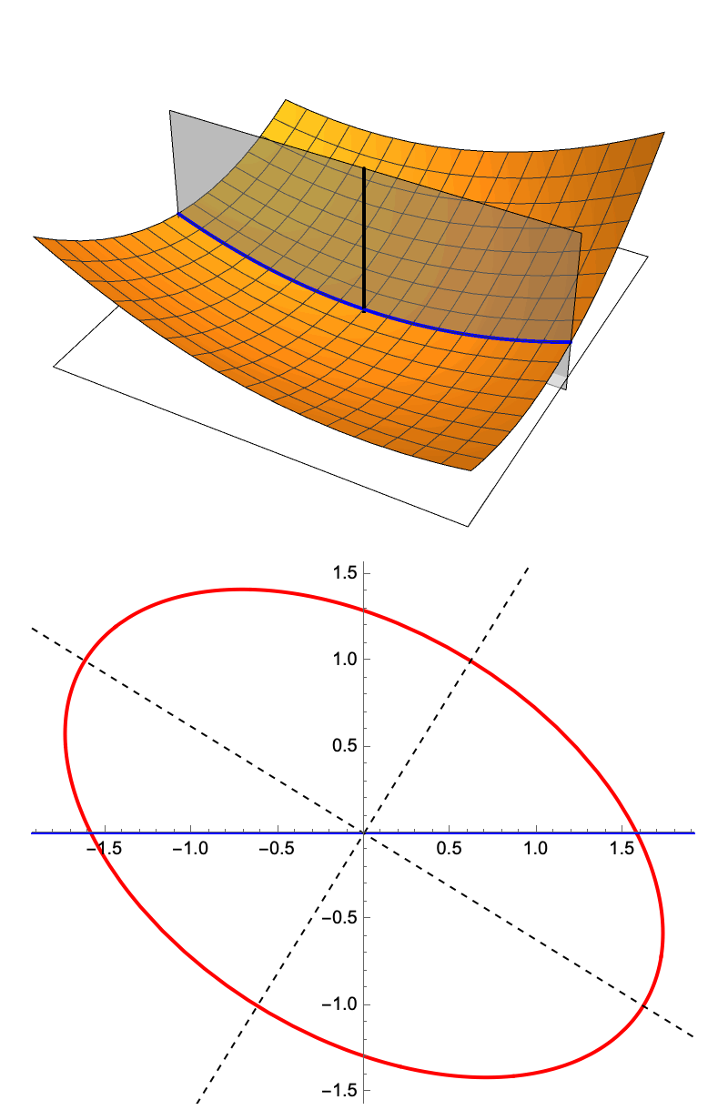
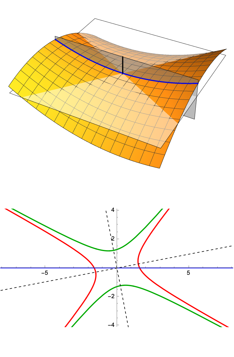
To do this, we will start by examining the curves we get if we slice the surface with a plane that contains the normal to the surface at P, as in the diagrams on the upper right. These curves are known as normal sections of the surface. Each such curve (blue in the diagram) is either a parabola or a straight line:
z(ρ, θ) = ½ [A(cos θ)2 + 2B cos θ sin θ + C(sin θ)2] ρ2
Here θ is the angle the slicing plane makes with the x-axis, and ρ is the horizontal distance measured from the z-axis.
We can quantify these parabolas’ curvature, κ, by computing the rate at which a unit-length tangent to the curve is changing direction. For a perfect circular arc of radius R, the curvature defined this way is just 1/R. For a parabola of the form z = ½b x2, it is equal to b at x = 0. And where the parabola we obtain by slicing through our quadratic surface passes through the point P, the curvature is equal to:
κ(θ) = A(cos θ)2 + 2B cos θ sin θ + C(sin θ)2
In the diagrams on the lower right, the reciprocal of the square root of the absolute value of the curvature is plotted as the distance from the origin for different values of θ, with red for positive curvature and green for negative curvature. A plot like this is known as the Dupin indicatrix of the surface at this point. If the surface is simply a quadratic, like the ones shown here, the Dupin indicatrix corresponds to contours z = ±½ in the function z(x, y) that gives the distance of the surface from the normal plane. These contours are conic sections: there are red and green hyperbolas where the curvature changes sign, and a red ellipse where the curvature remains positive.
If we define S0 to be the matrix:
S0 =
A B B C
then we can write the quadratic expression for z, and the curvature along the slice, as:
z(x, y) = ½ (x, y)T S0 (x, y)
κ(θ) = (cos θ, sin θ)T S0 (cos θ, sin θ)
The curvature will reach maximum and minimum values when the vector (cos θ, sin θ) is an eigenvector of the matrix S0, and the curvature itself will be the corresponding eigenvalue.
The dashed lines in the plots show the directions of the eigenvectors. But we don’t need to find the eigenvectors to know that the eigenvalues, κ1 and κ2, will be the two roots of the characteristic polynomial of S0:
det(S0 – κ I) = κ2 – (A + C) κ + (A C – B2) = 0
And we don’t need to solve this quadratic equation explicitly to know that the product of its two roots is equal to the constant term in the quadratic:
K = κ1 κ2 = A C – B2 = det(S0)
We call κ1 and κ2 the principal normal curvatures of the surface at point P, and we claim that their product is the Gaussian curvature, K, of the surface at P.
In fact, this is the original definition of Gaussian curvature, and the most common way of defining it when talking about embedded surfaces. It’s not hard to see that this will agree with our earlier definition in the case of a sphere, since every curve produced by a normal slice through a sphere of radius a will have curvature 1/a, so the product of κ1 and κ2 along any two slices will be 1/a2.
We can show that the definition of K as the product of the principal curvatures κ1 and κ2 agrees, in general, with our earlier definition of K in terms of the circumference of a circle.
To proceed, we will need to know the geodesic curves on our quadratic surface, or rather, we will need to approximate them with polynomial curves, well enough to compute the limiting behaviour of the circumference of a small circle. We will start by making use of a “canonical representation” of a curve in three-dimensional space with a given curvature, κ, rate of change of curvature dκ/ds, and torsion, τ, at some point. A curve with these properties can be approximated with three cubic polynomials in the arc length, s, measured from the point:[2]
G(s) = (s – (κ2/6) s3, (κτ/6) s3, (κ/2) s2 + ((dκ/ds)/6) s3)
This curve has a tangent at s = 0 that points along the x-axis, while the instantaneous rate of change of the tangent vector at s = 0 is a vector of length κ pointing along the z-axis. The torsion, τ, is the rate at which the plane of the curve is rotating around the curve.
Note that s is not precisely the arc length of this curve, but if we compute the squared length of the tangent with respect to s, it is equal to 1 plus terms of order 3 and 4 in s:
|G'(s)|2 = 1 + (dκ/ds) κ s3 + (((dκ/ds)2 + κ4 + κ2 τ2)/4) s4
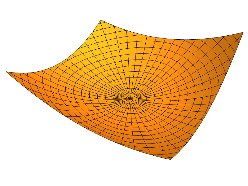 |
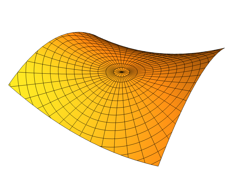 |
We want to find the geodesic curves that pass through the origin at an angle of θ with the x-axis, and whose curvature is given by the function κ(θ) that we computed earlier. We can set dκ/ds at the start of the curve to zero by symmetry, set τ to a function τ(θ) yet to be determined, and then rotate the whole curve G(s) around the z-axis so its tangent at s = 0 points in the correct direction.
In order to make the curve a good approximation to a geodesic for our quadratic surface, we will use the fact that along a geodesic, the curvature vector (the second derivative with respect to arc length) is parallel or antiparallel to the surface normal[3] and hence orthogonal to the tangents to the curves of varying θ (which lie within the surface). If we call our rotated curve Gθ(s), we find that to the lowest order in s:
Gθ''(s) · dGθ(s)/dθ ≈ ½ κ(θ) (κ'(θ) + 2 τ(θ)) s2
We can make this approximation zero by setting:
τ(θ) = –½κ'(θ) = (A – C) cos θ sin θ + B ((sin θ)2 – (cos θ)2)
It’s not surprising that the torsion is proportional to the derivative of the curvature, since the curvature reaches its maximum and minimum values when the plane slicing the surface is a plane of symmetry, and we would expect the geodesics there to be planar, i.e. with zero torsion.
Having chosen the torsion this way, we then find that up to order s3:
|dGθ(s)/dθ| ≈ s – (1/6)(A C – B2) s3
which tells us that the circumference of a circle of radius r in our quadratic surface, centred at the origin, will be:
Circumference(r) ≈ 2 π r – (π/3)(A C – B2) r3
and that
K = (3/π) limr → 0 (2 π r – Circumference(r)) / r3 = A C – B2
in agreement with our previous calculation that gave K as the product of the principal curvatures.
The images on the right show geodesics through the origin, and circles around the origin, for quadratic surfaces of positive (top) and negative (bottom) Gaussian curvature.
One of the most common ways to describe a surface embedded in three-dimensional space is by specifying its three Cartesian coordinates (x, y, z) as functions of two parameters, say u and v:
x(u, v) = (x(u, v), y(u, v), z(u, v))
We have seen how to compute the Gaussian curvature at a single point on a quadratic surface that we described in a carefully chosen Cartesian coordinate system, but it turns out not to be much harder to adopt the same computation to an arbitrary point on a parameterised surface (assuming, as always, that the relevant functions are sufficiently smooth for all the derivatives we need to exist).
We start by defining two matrices that are associated with each point on the surface x(u, v):
g(u, v) =
xu · xu xu · xv xu · xv xv · xv S(u, v) =
xuu · n xuv · n xuv · n xvv · n
where the symbol · is the usual Euclidean dot product between vectors, and we have introduced abbreviations for the following vectors at each point:
xu = ∂ux(u, v) is a tangent vector to the curve of varying u
xv = ∂vx(u, v) is a tangent vector to the curve of varying v
n = xu × xv / |xu × xv| is a unit-length normal to the surface
xuu = ∂u,ux(u, v) is the instantaneous rate of change of xu along the curve of varying u
xuv = ∂u,vx(u, v) = ∂v,ux(u, v) is the instantaneous rate of change of xu along the curve of varying v (and vice versa)
xvv = ∂v,vx(u, v) is the instantaneous rate of change of xv along the curve of varying v
The first of these matrices, g, is called the metric tensor or the first fundamental form, and S is known as the second fundamental form.
The metric, g, can be used to compute the dot product between two vectors, say a and b, that lie in the tangent plane to the surface, given their coordinates in the basis {xu, xv}:
a = au xu + av xv
b = bu xu + bv xv
a · b = (au, av)T g (bu, bv)
The second fundamental form, S, captures the same kind of quadratic Taylor series for the perpendicular distance from the tangent plane to the surface that we described with the matrix S0:
Perpendicular distance from tangent plane at P=x(uP,vP), to a nearby point on the surface, x(u,v)
≈ ½ (u – uP, v – vP)T S (u – uP, v – vP)
In fact, S0 is precisely what S would be if we chose parameters for the surface that corresponded to a Cartesian grid in the tangent plane at P.
But since we can obtain the Gaussian curvature, K, as the determinant of S0, we can also obtain it from the determinant of S, along with a factor that accounts for the change of basis between the vectors {xu, xv}, associated with the parameters u and v, and the orthonormal basis associated with the Cartesian coordinates we used when discussing S0.
Suppose the matrix M takes the coordinates of a vector in an orthonormal basis for the tangent plane, and gives us coordinates in the basis {xu, xv}. Then we can use the fact that g gives us the dot product in terms of the latter coordinates to write:
a · b = (au, av)T g (bu, bv) = (M (ax, ay))T g (M (bx, by)) = (ax, ay)T (MT g M) (bx, by)
where (ax, ay), (bx, by) are the coordinates of the vectors a and b in the orthonormal basis. But we also have:
a · b = (ax, ay)T I (bx, by)
where I is the 2×2 identity matrix. For this to hold for all pairs of vectors a and b, we must have:
MT g M = I
from which it follows that:
det(MT) det(g) det(M) = det(I)
det(M)2 = 1 / det(g)
But the same change of basis matrix M applies to S and S0:
S0 = MT S M
which lets us write the Gaussian curvature as:
K = det(S0) = det(M)2 det(S) = det(S) / det(g)
We can check this with a calculation for a sphere of radius a embedded in three-dimensional space, with the usual polar coordinates as the parameters:
x(u, v) = a (sin u cos v, sin u sin v, cos u)
xu = a (cos u cos v, cos u sin v, –sin u)
xv = a (–sin u sin v, sin u cos v, 0)
n = (sin u cos v, sin u sin v, cos u)
xuu = a (–sin u cos v, –sin u sin v, –cos u)
xuv = a (–cos u sin v, cos u cos v, 0)
xvv = a (–sin u cos v, –sin u sin v, 0)
g(u, v) =
xu · xu xu · xv xu · xv xv · xv =
a2 0 0 a2 (sin u)2 S(u, v) =
xuu · n xuv · n xuv · n xvv · n =
–a 0 0 –a (sin u)2
K = det(S) / det(g) = [a2 (sin u)2 ] / [a4 (sin u)2] = 1/a2
We’ve seen how to compute the Gaussian curvature for a surface embedded in three-dimensional Euclidean space, but we know, from our definition of the curvature in terms of the geometry of a circle within the space, that Gaussian curvature is an intrinsic property of the two-dimensional space itself. So we ought to be able to compute it without making use of any information about the embedding, and in situations where the space of interest simply isn’t embedded in any higher-dimensional space at all.
The intrinsic geometry of a space is determined by its metric, g. We described how g can be computed for an embedded surface in the last section, where the geometry of the surface is induced by the geometry of the three-dimensional space in which it sits, but in the context of intrinsic geometry the metric is simply stated as part of the definition of the space. So our goal will be to compute the Gaussian curvature from the metric alone.
There is a substantial body of mathematics dealing with various measures of intrinsic curvature in spaces of arbitrary dimension, much of which was first developed in the nineteenth century, and later found a role in the twentieth century physics of General Relativity. I sketched some of the essential ideas needed for GR in a short article that covers the notions of parallel transport and the Riemann curvature tensor, and these concepts are well worth studying both for their physical applications and for a deeper understanding of the geometry itself. But for our purposes all we really need is a formula for the Gaussian curvature in terms of the metric.
We will approach this by seeking an equation that describes the geodesic curves in a space with a given metric, g(u, v). Suppose we have a curve G(λ) from the point P with coordinates (uP,vP) to the point Q with coordinates (uQ,vQ):
G(λ) = (uG(λ), vG(λ))
G(0) = (uG(0), vG(0)) = (uP,vP)
G(1) = (uG(1), vG(1)) = (uP,vP)
Here uG(λ) and vG(λ) are whatever functions give the coordinates of G(λ), and λ is a parameter that ranges from 0 to 1 along the curve.
If G(λ) is a geodesic, then any curve from P to Q will be longer than G(λ). Specifically, suppose we have functions uδ(λ) and vδ(λ) that satisfy:
uδ(0) = uδ(1) = 0
vδ(0) = vδ(1) = 0
and we add multiples of these functions to the coordinates of G(λ) to obtain a family of curves from P to Q, with a parameter μ specifying the different curves within this family:
cμ(λ) = (uG(λ) + μ uδ(λ), vG(λ) + μ vδ(λ))
c0(λ) = G(λ)
The length of any particular curve in this family will be given by:
L(μ) = ∫01 √[cμ'(λ)T g cμ'(λ)] dλ
For the sake of brevity we simply write g for the metric, but note that we mean g(cμ(λ)), i.e. we must evaluate the metric, which is a function of the coordinates u and v, along the curve cμ(λ), which makes the metric a function of both μ and λ.
(We introduced the metric as a way of computing the dot product between vectors in the tangent plane to a surface embedded in three-dimensional space, but we haven’t talked about the precise meaning of a “vector” when the two-dimensional curved space isn’t embedded in any larger space. For our present purposes, we will simply note that this way of computing the length of a curve is consistent with the way we introduced the metric. The dot product of any vector with itself is the squared length of that vector, so the square root of the dot product with itself of the vector tangent to a curve, with respect to the parameter λ, gives the rate of change ds/dλ of arc length s along the curve with respect to λ, and this integral will give the total length of the curve. The article on General Relativity mentioned earlier delves into exactly what a tangent vector means in the context of intrinsic geometry.)
If c0(λ) = G(λ) is a geodesic, the function L(μ) that gives the length of each curve in this family will have a minimum at μ = 0. We would expect L(μ) to be a differentiable function, with a derivative of zero at its minimum:
L'(0) = 0
What’s more, we expect this to be true whatever functions we choose for uδ(λ) and vδ(λ), so long as they are zero at their endpoints. This amounts to saying that however we choose a family of curves from P to Q that includes the geodesic G(λ), the geodesic will always be the shortest, at least compared to other curves that only differ from it by a small amount. (In spaces that are not simply connected, there might be several geodesics that join the same two points, only one of which will be the shortest.)
We want to find the derivative of L(μ). Starting with the derivatives with respect to μ of some pieces of the integral, we have:
dcμ(λ)/dμ = (uδ(λ), vδ(λ))
dcμ'(λ)/dμ = (uδ'(λ), vδ'(λ))
dg/dμ = ∂g/∂u uδ(λ) + ∂g/∂v vδ(λ)
d [cμ'(λ)T g cμ'(λ)] / dμ = 2 (uδ'(λ), vδ'(λ))T g cμ'(λ) + cμ'(λ)T (∂g/∂u uδ(λ) + ∂g/∂v vδ(λ)) cμ'(λ)
L'(μ) = ∫01 (d √[cμ'(λ)T g cμ'(λ)] / dμ) dλ
= ∫01 (d [cμ'(λ)T g cμ'(λ)] / dμ) / (2 √[cμ'(λ)T g cμ'(λ)]) dλ
We can apply the formula for integration by parts:
∫01 f '(λ) g(λ) dλ = f(1) g(1) – f(0) g(0) – ∫01 f(λ) g'(λ) dλ
to terms multiplied by uδ'(λ) or vδ'(λ), to rewrite the last integral as:
L'(μ) = ∫01 { – (uδ(λ), vδ(λ))T d/dλ [g cμ'(λ) / √[cμ'(λ)T g cμ'(λ)]] + ½ cμ'(λ)T (∂g/∂u uδ(λ) + ∂g/∂v vδ(λ)) cμ'(λ) / √[cμ'(λ)T g cμ'(λ)] } dλ
If we evaluate this at μ = 0, it should be zero regardless of choices we make for uδ(λ) and vδ(λ), which can only be true if both those functions appear in the integral multiplied by factors that are zero for all values of λ. Recall that c0 is equal to G, so we have:
– (1, 0)T d/dλ [g G'(λ) / √[G'(λ)T g G'(λ)]] + ½ G'(λ)T (∂g/∂u) G'(λ) / √[G'(λ)T g G'(λ)] = 0
– (0, 1)T d/dλ [g G'(λ) / √[G'(λ)T g G'(λ)]] + ½ G'(λ)T (∂g/∂v) G'(λ) / √[G'(λ)T g G'(λ)] = 0
We can divide both equations by √[G'(λ)T g G'(λ)], multiply by –1, and then use:
√[G'(λ)T g G'(λ)] = ds/dλ
1/ √[G'(λ)T g G'(λ)] = dλ/ds
to change all derivatives with respect to λ into derivatives with respect to arc length, s. We also redefine G, uG and vG to be functions of s rather than of λ, to keep the notation simple.
(1, 0)T d/ds [g G'(s)] – ½ G'(s)T (∂g/∂u) G'(s) = 0
(0, 1)T d/ds [g G'(s)] – ½ G'(s)T (∂g/∂v) G'(s) = 0
If we write x1 for uG(s) and x2 for vG(s), write the components of the metric as gij, and use the Einstein summation convention of summing over {1,2} for any repeated index in a product, we can write both these equations as:
gij d2xj/ds2 + [∂gij/∂xk – ½ ∂gjk/∂xi] (dxj/ds) (dxk/ds) = 0
where the index i is either 1 or 2 for the two equations, and j and k are summed over {1,2}. The expression in brackets can be replaced by something more symmetrical, where we take the average of the first term and a version of it with j and k swapped:
Γijk = ½(∂gij/∂xk + ∂gik/∂xj – ∂gjk/∂xi)
This is not identical to the expression in brackets, but when we sum over j and k in the equation the sum turns out to be exactly the same, because (dxj/ds) (dxk/ds) is symmetrical when we swap j and k. The equations can then be written as:
gij d2xj/ds2 + Γijk (dxj/ds) (dxk/ds) = 0
The Γijk are known as the Christoffel symbols of the first kind. It would make no difference to any of our calculations if we used the original expression in brackets instead, but using the Christoffel symbols is normal practice, and it would risk confusion if we didn’t follow it.
The most common version of the geodesic equations is:
d2xi/ds2 + Γijk (dxj/ds) (dxk/ds) = 0
where we have removed the metric multiplying the second derivative term by multiplying through by the inverse of the metric, g–1, whose components are usually written as gij, and we define Christoffel symbols of the second kind as:
Γijk = gim Γmjk = ½ gim (∂gmj/∂xk + ∂gmk/∂xj – ∂gjk/∂xm)
To check that what we’ve done so far is correct, let’s compute the Christoffel symbols for the simplest curved space: a sphere of radius a, with the parameters u and v as the co-latitude (angle from the north pole) and longitude.
g(u, v) =
a2 0 0 a2 (sin u)2 Γ1(u, v) =
0 0 0 –a2 sin u cos u Γ2(u, v) =
0 a2 sin u cos u a2 sin u cos u 0 g–1(u, v) =
a–2 0 0 a–2 (sin u)–2 Γ1(u, v) =
0 0 0 –sin u cos u Γ2(u, v) =
0 cot u cot u 0
We will sneak back into three-dimensional space and write the Cartesian coordinates for a family of geodesics that pass through the point (a, 0, 0) and make an angle θ with the equator. To move a distance s along one of these geodesics, we just rotate by the angle s/a from our starting point towards a point where the geodesic reaches its maximum latitude, (0, a cos(θ), a sin(θ)):
Gxyz(s) = cos(s/a) (a, 0, 0) + sin(s/a) (0, a cos(θ), a sin(θ)) = a (cos(s/a), cos(θ) sin(s/a), sin(θ) sin(s/a))
The co-latitude and longitude are then given by:
uG(s) = acos[sin(θ) sin(s/a)]
vG(s) = atan[cos(θ) tan(s/a)]
The first derivatives with respect to s are:
uG'(s) = –sin(θ) cos(s/a) / (a [1 – sin(θ)2 sin(s/a)2]1/2)
vG'(s) = cos(θ) / (a [1 – sin(θ)2 sin(s/a)2])
and the second derivatives are:
uG''(s) = sin(θ) cos(θ)2 sin(s/a) / (a2 [1 – sin(θ)2 sin(s/a)2]3/2)
vG''(s) = 2 cos(θ) sin(θ)2 sin(s/a) cos(s/a) / (a2 [1 – sin(θ)2 sin(s/a)2]2)
Along these geodesics, the Christoffel symbols of the second kind become:
Γ1(s) =
0 0 0 –sin(θ) sin(s/a) √[1 – sin(θ)2 sin(s/a)2] Γ2(s) =
0 sin(θ) sin(s/a) / √[1 – sin(θ)2 sin(s/a)2] sin(θ) sin(s/a) / √[1 – sin(θ)2 sin(s/a)2] 0
It’s not hard to check that:
uG''(s) + Γ122(s) vG'(s)2 = 0
vG''(s) + 2 Γ212(s) uG'(s) vG'(s) = 0
which confirms that uG(s), vG(s) satisfy the geodesic equations.
Our aim now is to compute the Gaussian curvature for any metric, by finding the coefficient of the s3 term in the circumference of a circle with a geodesic radius of s. To do this, we will need a Taylor series for the geodesics through a point to third-order in s. The geodesic equation gives us the second derivatives in terms of the first derivatives, and we can differentiate again to get the third derivatives.
d2xi/ds2 = –Γijk (dxj/ds) (dxk/ds) d3xi/ds3 = –∂Γijk/∂xm (dxj/ds) (dxk/ds) (dxm/ds) – 2 Γijk (d2xj/ds2) (dxk/ds) = –∂Γijk/∂xm (dxj/ds) (dxk/ds) (dxm/ds) + 2 Γijk Γjpq (dxp/ds) (dxq/ds) (dxk/ds) = [2 Γijk Γjpq – ∂Γipk/∂xq] (dxp/ds) (dxq/ds) (dxk/ds)
If we abbreviate the first derivatives by writing:
Xi = [dxi/ds]s = 0
then the third-order Taylor series for the geodesic can be written:
xi ≈ xiP + Xi s – ½ Γijk Xj Xk s2 + (1/6) [2 Γijk Γjpq – ∂Γipk/∂xq] Xp Xq Xk s3
where the Christoffel symbols and their derivatives are also evaluated at s = 0.
By rotating the tangent to the geodesic at the start, a point that lies at a distance of s along the curve will sweep out a circle of constant geodesic radius. We want to find the length of the tangent to that circle, with respect to the angle of rotation of the geodesic’s initial tangent. But rather than explicitly writing the components of the initial tangent, Xi, as functions of a direction angle θ, we will use the fact that their derivatives with respect to θ must be the components of a unit-length vector orthogonal to the tangent. In Euclidean coordinates, this would simply be a matter of noting that the counter-clockwise unit vector orthogonal to some unit vector (X, Y) is (–Y, X), but because we are dealing with general coordinates, we need to use a slightly fancier formula:
Zα = –εαβ gβγ Xγ / √det(g) where ε =
0 1 –1 0
The symbol ε here is called the Levi-Civita symbol. Given any tangent vector X whose components are rates of change of the u, v coordinates, the vector Z will be orthogonal to it, and of the same length.
Taking the derivative of the geodesic with respect to the initial tangent components Xα gives us:
dxi/dXα ≈ δiα s – Γiαk Xk s2 + (1/6) [4 Γijq Γjαp + 2 Γijα Γjpq – 2 ∂Γiαq/∂xp – ∂Γipq/∂xα] Xp Xq s3
We then obtain the tangent vector to the circle by multiplying by Zα (with the implied sum from the repeated index α):
dxi/dθ ≈ Z i s – Γiαk Xk Zα s2 + (1/6) [4 Γijq Γjαp + 2 Γijα Γjpq – 2 ∂Γiαq/∂xp – ∂Γipq/∂xα] Xp Xq Zα s3
We compute the squared length of this tangent to the circle with the metric, but we can’t simply use the metric at the start of the geodesic; we need to use a Taylor series in s.
gij(s) ≈ gij(0) + ∂gij/∂xp Xp s + ½ [∂2gij/(∂xp ∂xq) – ∂gij/∂xr Γrpq] Xp Xq s2
|dG/dθ|2 = gij(s) dxi/dθ dxj/dθ
The lowest-order term in the squared length is the second-order term in s, which is:
The coefficient is 1, because Z is a unit-length vector.
gij(0) Z i Z j s2 = s2
The third-order term is the sum of:
Note that multiplying Christoffel symbols of the second kind by the metric lowers the first index and converts them back to Christoffel symbols of the first kind. Because the expression in brackets is antisymmetric (i.e. it changes sign) when α and β are exchanged, summing it with the symmetric expression Zα Zβ gives zero.
[∂gβα/∂xk – 2 giβ(0) Γiαk] Xk Zα Zβ s3
= [∂gβα/∂xk – 2 Γβαk] Xk Zα Zβ s3
= [∂gαk/∂xβ – ∂gβk/∂xα] Xk Zα Zβ s3
= 0
The fourth-order term is the sum of:
[(1/3) giβ(0) (4 Γijq Γjαp + 2 Γijα Γjpq – 2 ∂Γiαq/∂xp – ∂Γipq/∂xα)
+ gij(0) Γiαp Γjβq
– 2 ∂gαj/∂xp Γjβq
+ ½(∂2gαβ/(∂xp ∂xq) – ∂gαβ/∂xj Γjpq)] Xp Xq Zα Zβ s4
= [(1/3) (4 Γβjq Γjαp + 2 Γβjα Γjpq – 2 giβ(0) ∂Γiαq/∂xp – giβ(0) ∂Γipq/∂xα)
+ (Γjαp – 2 ∂gαj/∂xp) Γjβq
+ ½(∂2gαβ/(∂xp ∂xq) – ∂gαβ/∂xj Γjpq)] Xp Xq Zα Zβ s4
= – (1/3) (Γjαq Γjβp – Γjpq Γjβα + ∂Γβpq/∂xα – ∂Γβαq/∂xp) Xp Xq Zα Zβ s4
The combination of Christoffel symbols and their derivatives that appears here:
Rβqαp = Γjαq Γjβp – Γjpq Γjβα + ∂Γβpq/∂xα – ∂Γβαq/∂xp
is known as the Riemann curvature tensor. Given the four indices, in two dimensions it has 16 components, but it is so symmetrical that 12 of them are zero, and the other four all have the same absolute value, so it is essentially described by a single number. Specifically, swapping either the first two indices (β ↔ q) or the last two indices (α ↔ p) changes the sign, and swapping the first two with the last two (βq ↔ αp) leaves the value unchanged.
We will define the other tensor we summed this against as S:
Sβqαp = Xp Xq Zα Zβ
= Xp Xq εαγ gγδ Xδ εβη gησ Xσ / det(g)
While S itself depends on the vector X, if we add up four copies where we swap indices and change signs as follows, we find that:
Sβqαp – Sqβαp – Sβqpα + Sqβpα = ½ (XT g X)2 (Hβqαp – Hqβαp – Hβqpα + Hqβpα)
where H is defined as:
Hβqαp = gpq gαβ
Since X is always chosen to be a unit-length vector, the factor on the right-hand side just becomes ½. If we multiply both sides of this equation by Rβqαp, we get:
Rβqαp Sβqαp – Rβqαp Sqβαp – Rβqαp Sβqpα + Rβqαp Sqβpα = ½ (Rβqαp Hβqαp – Rβqαp Hqβαp – Rβqαp Hβqpα + Rβqαp Hqβpα)
The second, third and fourth terms on each side of the equation now have different ordering of the indices on the two tensors, but we can use the symmetries of the Riemann tensor to make its indices match the other tensor in each case, while also removing all the minus signs:
Rβqαp Sβqαp + Rqβαp Sqβαp + Rβqpα Sβqpα + Rqβpα Sqβpα = ½ (Rβqαp Hβqαp + Rqβαp Hqβαp + Rβqpα Hβqpα + Rqβpα Hqβpα)
Now that the order of the indices match, if we sum over all values for all indices we just get four identical sums on each side of the equation:
4 Rβqαp Sβqαp = 2 Rβqαp Hβqαp
So our fourth order term becomes, independent of X:
– (1/6) gpq gαβ Rβqαp s4
Our calculation so far has been for the squared length of the tangent vector dxi/dθ:
|dxi/dθ|2 ≈ s2 – (1/6) gpq gαβ Rβqαp s4
but we want the length itself:
|dxi/dθ| ≈ s – (1/12) gpq gαβ Rβqαp s3
It follows that the Gaussian curvature is given by:
K = ½gpq gαβ Rβqαp
For the case of a sphere, we already have the Christoffel symbols, and it is not too hard to find the Riemann tensor, whose four non-zero components are:
R1212 = R2121 = a2 (sin u)2
R1221 = R2112 = –a2 (sin u)2
The components of the inverse metric are:
g11 = a–2
g22 = a–2 (sin u)–2
g12 = g21 = 0
So we have:
K = ½(g22 g11 R1212 + g11 g22 R2121 + g12 g21 R1221 + g21 g12 R2112) = 1/a2
as expected.
[1] Theory and Problems of Differential Geometry, Martin Lipschutz, Schaum’s Outline Series, McGraw-Hill 1969.
[2] Lipschutz, op. cit., page 83.
[3] Lipschutz, op. cit., page 233, equation (11.3).
[4] Lipschutz, op. cit., page 234, Theorem 11.7.
[5] Lipschutz, op. cit., page 256, solved problem 11.26.
[6] Lipschutz, op. cit., page 257, solved problem 11.27.
[7] Seguin B, Chen Y-c, Fried E. 2021 “Bridging the gap between rectifying developables and tangent developables: a family of developable surfaces associated with a space curve.” Proc. R. Soc. A 477: 20200617. https://doi.org/10.1098/rspa.2020.0617
[8] Lipschutz, op. cit., page 187.
[9] Lipschutz, op. cit., page 203, equation (10.7).
[10] Lipschutz, op. cit., page 188, Theorem 9.18.
[11] Bäcklund and Darboux Transformations: Geometry and Modern Applications in Soliton Theory, C. Rogers and W. K. Schief, Cambridge University Press, 2002. Section 1.3.1.
[12] Rogers and Schief, op. cit., Section 1.4.4.
[13] Rogers and Schief, op. cit., page 27, equation (1.52).
[14] Lipschutz, op. cit., page 180, equation (9.17).
[15] Coxeter, H. S. M. “The Non-Euclidean Symmetry of Escher’s Picture ‘Circle Limit III’” Leonardo, Vol. 12, No. 1 (Winter, 1979), pp. 19-25. Online at https://www.jstor.org/stable/1574078.