
In the interior of a solid ball of matter with uniform density, the Newtonian gravitational potential takes the simple form:
Ψ(r) = 2 π G ρ (⅓ r2 – R2)
where G is the Newtonian gravitational constant, ρ is the density, and R is the radius of the ball.
Of course this is just a toy model that is quite different from real astronomical bodies, whose density will usually vary significantly with depth unless they are quite small — and if they are small they are less likely to be spherical.
What about an ellipsoid, rather than a spherical ball? It turns out that the potential in the interior of an ellipsoid with uniform density again takes on about the simplest form possible, given that the shape is no longer radially symmetrical:
Ψ(x, y, z) = 2 π G ρ (A x2 + B y2 + C z2 + D)
We will prove this result and find the values of the four coefficients in this formula in terms of the dimensions of the ellipsoid. We will then examine some of the consequences of this for slightly more complicated systems, such as a uniformly spinning body made of a fluid of constant density.
Most of the results discussed here are centuries old, and I will not make any attempt to give detailed attributions. There is a wonderful survey of the whole topic by Chandrasekhar[1] that traces some of the history as well as delving deeply into the mathematical physics. [Our notation will be largely the same as Chandrasekhar, but our coefficients A, B, C are half what Chandrasekhar calls A1, A2, A3, and they sum to 1 rather than 2.]
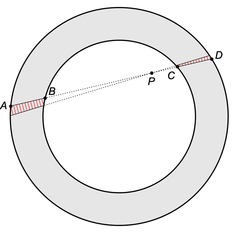
Consider a shell of uniform density, whose boundaries are two concentric spheres. Newton gave a simple argument that a body located anywhere inside this shell will experience no gravitational force from the shell.
Suppose the body is located at point P in the diagram on the left. If we consider the material of the shell that lies within a narrow double cone with its apex at P, it can be subdivided into slices that lie at an equal distance r from P. The amount of matter in each such slice will be proportional to r2 dr, but the inverse-square law of gravity means the force at P is proportional to 1/r2, and hence the total force from each slice is independent of r and just proportional to its thickness, dr.
This means the total force at P in the direction of B is proportional to the distance AB, while the total force in the direction of C is proportional to the distance CD. But because the boundaries of the shell are concentric spheres we always have AB = CD, so there are equal and opposite forces at P that (in the limit of an infinitesimal cone) cancel out exactly. By summing over infinitesimal cones and infinitesimal slices, we can account for all the matter in the shell this way, so the effect of the entire shell is that there is zero net force, for any choice of P.
If there is no gravitational force inside the shell, the gravitatitional potential, Ψ, must be constant. That means the potential everywhere inside the shell will be equal to the potential at the centre.
For an infinitesimally thin shell with a radius S and a uniform surface density of σ, the potential at the centre, and hence the potential throughout the interior, is:
Ψshell, int(S, σ, r)
= –G M / S
= –G (4 π S2 σ) / S
= –4 π G σ S
We can confirm (and extend) this result with a direct computation. The potential at some point P at a distance r from the centre of an infinitesimal shell of radius S and surface density σ can be found by integrating over the surface.
Ψshell(S, σ, r) = –2 π G σ S2 ∫0π sin θ / √[S2 + r2 – 2 S r cos θ] dθ
Here θ is the angle between a ray from the centre of the shell that passes through the point P and a ring of matter on the shell that is equidistant from P. The ring of matter has a radius of S sin θ and a thickness measured along the surface of the shell of S dθ, and the distance from P is given by the denominator in the integral above.
With a change of variable to u = cos θ we have:
Ψshell(S, σ, r) = –2 π G σ S2 ∫–11 1 / √[S2 + r2 – 2 S r u] du
= (2 π G σ S / r) (√[S2 + r2 – 2 S r u]) |–11
= (2 π G σ S / r) (√[S2 + r2 – 2 S r] – √[S2 + r2 + 2 S r])
= (2 π G σ S / r) (|S – r| – |S + r|)
This gives us, for the interior of the shell where r ≤ S, and the exterior where r ≥ S:
Potential for an infinitesimal spherical shell of radius S and uniform surface density σ
Ψshell, int(S, σ, r) = –4 π G σ S
Ψshell, ext(S, σ, r) = –4 π G σ S2 / r
So, as we showed previously, the potential inside the shell is constant (and hence a test particle there would experience no gravitational force) while the potential outside the shell is the same as that due to a point mass (of the same mass as the whole shell) located at the centre of the shell.
We can now compute the potential inside or outside a solid ball of uniform density ρ and radius R, by integrating the contribution from a continuum of shells whose radius S ranges from 0 to R.
If the point of interest lies at a distance r from the centre of the ball, then for the interior case, where r ≤ R, the point lies in the exterior of all the shells with radius ranging from 0 to r, but in the interior of those with radius ranging from r to R:
Ψball, int(R, ρ, r) = ∫0r Ψshell, ext(S, ρ, r) dS + ∫rR Ψshell, int(S, ρ, r) dS
= –4 π G ρ (∫0r (S2 / r) dS + ∫rR S dS)
= –4 π G ρ (⅓ r2 + ½ R2 – ½ r2)
= 2 π G ρ (⅓ r2 – R2)
For the exterior case, where r ≥ R, the point of interest lies in the exterior of all the shells:
Ψball, ext(R, ρ, r) = ∫0R Ψshell, ext(S, ρ, r) dS
= –4 π G ρ ∫0R (S2 / r) dS
= –(4/3) π G ρ R3 / r
In the exterior case, the potential is the same as that of a point mass, of the same total mass as the ball, located at its centre.
In the interior case, the potential increases with the square of the distance from the centre, so the gravitational acceleration, which is the opposite of the gradient of the potential, is proportional to the distance from the centre. This means that a test particle dropped into a borehole in a solid sphere of uniform density would undergo simple harmonic motion like a weight on the end of a spring, a famous thought experiment that you can read much more about here.
Potential for a solid ball of radius R and uniform density ρ
Ψball, int(R, ρ, r) = 2 π G ρ (⅓ r2 – R2)
Ψball, ext(R, ρ, r) = –(4/3) π G ρ R3 / r
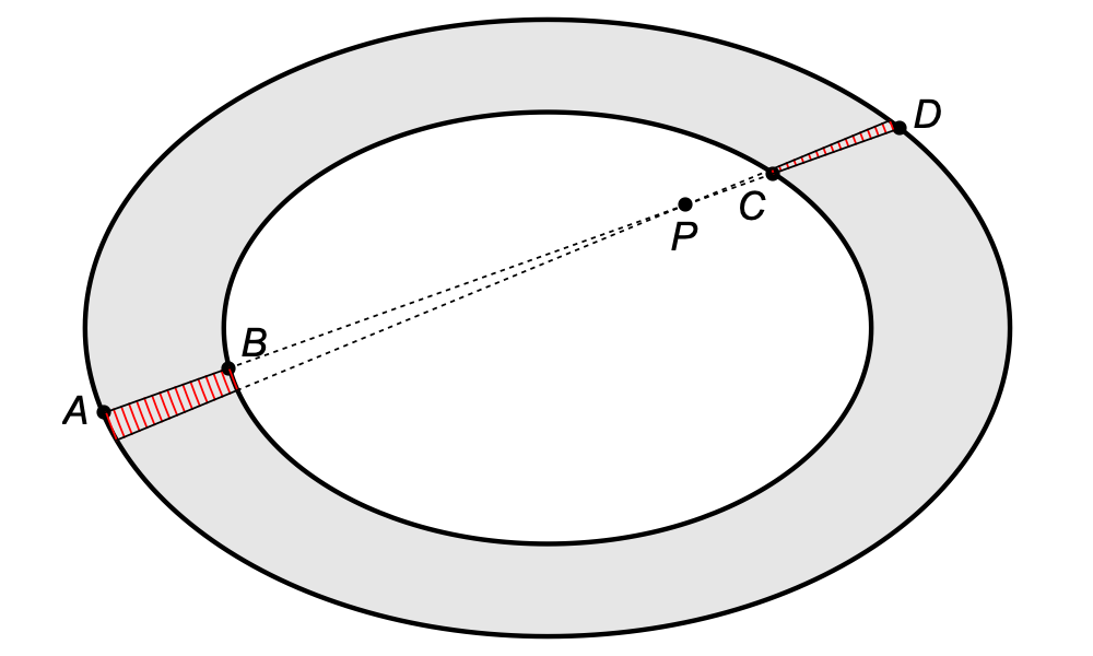
The same argument that shows that there is no net gravitational force on a body inside a spherical shell of uniform density works just as well for an ellipsoidal shell of uniform density — so long as the inner and outer boundaries of the shell are concentric, aligned along the same axes, and are similar ellipsoids (that is, they are the same shape apart from an overall scale factor).
If the shell meets those requirements, we can be sure that the distance AB in the diagram on the left will always equal the distance CD, because we can obtain the ellipsoidal shell by applying a suitable linear transformation to a spherical shell. A linear transformation will always multiply the lengths of any two parallel line segments by the same factor, so the pairs of equal distances from the spherical case will remain equal.
A shell like this is known as a homoeoid. Note that the thickness of a homoeoid, measured orthogonally to the surface, is not constant. This means that an infinitesimally thin ellipsoidal shell with a constant surface density, i.e. a fixed quantity of mass per unit area, will not be a homoeoid, and it will not exert zero net gravitational force in its interior. Of course we can still study infinitesimally thin homoeoids, but they will not have constant surface densities.
An ellipsoid with semi-axes of length a, b and c has a boundary that can be described (in a coordinate system with its origin at the centre of the ellipsoid and its axes aligned with those of the ellipsoid) by the quadratric equation:
x2/a2 + y2/b2 + z2/c2 = 1
We will assume that our ellipsoid has a uniform density of ρ.
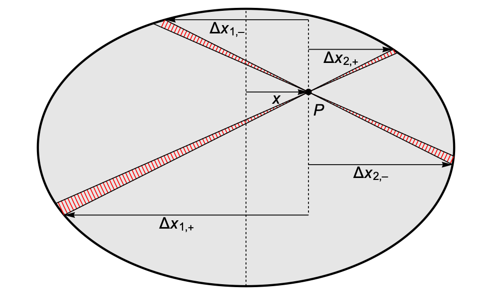
As with the ellipsoidal shell, we will consider the gravitational force at some point P due to the matter in a narrow double cone with its apex at P, but we will consider two such double cones at the same time, with the y- and z-components of the two cones’ direction vectors being the opposite of each other, as in the diagram on the left.
As we noted before, the amount of material in each slice of the cone at a given distance r is proportional to r2 dr, while the inverse-square law means the force is proportional to 1/r2. So the force due to each slice is just proportional to its thickness, dr, and the total force at P due to the matter in each cone will be proportional to the length of the cone.
It follows that the x-component of the force at P due to each cone is proportional to the extent of the cone in the x direction, Δx, where this is a signed quantity, with a force in the negative x direction when Δx is negative.
If P has coordinates (x, y, z), the four values of Δx are the roots of the two quadratic equations:
Q±(Δx) = (x + Δx)2 / a2 + (y ± β Δx)2 / b2 + (z ± γ Δx)2 / c2 – 1 = 0
The parameters β and γ determine the direction of the cones, while the sign determines which of the two double cones we are looking at.
We don’t need to explicitly solve these quadratics, because we don’t care about the individual values of Δx, just the sum of all four values. The sum of the two roots of any quadratic is simpler than the individual roots:
If Q2 Δx2 + Q1 Δx + Q0 = 0
then Δx1 + Δx2 = –Q1/Q2
For our particular quadratics, we have:
Q2 = 1 / a2 + β2 / b2 + γ2 / c2
Q1,± = 2 x / a2 ± 2 β y / b2 ± 2 γ z / c2
Δx1,+ + Δx2,+ + Δx1,– + Δx2,–
= –(Q1,+ + Q1,–) / Q2
= –4 x / (a2 Q2)
So the total x-component of the force at P due to the matter in all four cones is independent of y and z, and directly proportional to x. The constant of proportionality will vary with the direction of the cones, but it will not depend on P at all, so we can integrate over all directions for the cones, taking in all the material of the ellipsoid, to obtain a single constant.
The same analysis can be applied to the y-component and z-component of the force, with a different constant of proportionality for each axis. We will compute the constants themselves later, by a slightly different method, but what we have shown is that the gravitational force at P has components along each axis that are proportional to the displacement from the centre along that axis.
From that simple, linear relationship, it follows that the gravitational potential must take a simple quadratic form, which we can write as:
Ψ(x, y, z) = 2 π G ρ (A x2 + B y2 + C z2 + D)
Instead of trying to compute the gravitational potential at an arbitrary point in the interior directly, we will perform a couple of simpler calculations: finding the potential at the centre of the ellipsoid, which we will call Ψ0, and the potentials at the vertices of the ellipsoid, where the axes intersect the boundary, which we will call Ψa, Ψb and Ψc. Those four quantities will be all we need to find the four coefficients A, B, C and D.
To compute Ψ0, imagine sweeping a vector s = (sx, sy, sz) across a unit sphere with the same centre as the ellipsoid, and summing the potential due to the matter in a cone around s that subtends an infinitesimal solid angle ds and reaches from the centre to the boundary. The height of the cone, h0(s), will satisfy:
h0(s)2 sx2/a2 + h0(s)2 sy2/b2 + h0(s)2 sz2/c2 = 1
h0(s)2 = 1 / (sx2/a2 + sy2/b2 + sz2/c2)
The potential at the centre due to the matter in each cone can be found by integrating over the distance from the centre, r, from 0 to h0(s):
dΨ0 = (–G ρ ∫0h0(s) r2/r dr) ds
= –½ G ρ h0(s)2 ds
If we adopt standard polar coordinates where:
s = (sin θ cos φ, sin θ sin φ, cos θ)
ds = sin θ dφ dθ
we then have an integral for Ψ0:
Ψ0(a, b, c) = –½ G ρ ∫0π ∫02π sin θ / [sin2 θ cos2 φ / a2 + sin2 θ sin2 φ / b2 + cos2 θ / c2] dφ dθ
Before computing this for the generic case where none of the semi-axes are equal, suppose we have an ellipsoid of revolution, with two equal semi-axes, and choose the axes so that a = b. The integrand then becomes independent of φ, so we can replace that part of the integration by a factor of 2π, giving us:
Ψ0(a, a, c) = –π G ρ ∫0π sin θ / [sin2 θ / a2 + cos2 θ / c2] dθ
If a > c (an oblate spheroid), we can make the substitution:
tan α = √[a2/c2 – 1] cos θ
sec2 α dα = (1 + tan2 α) dα = –√[a2/c2 – 1] sin θ dθ
(1 + (a2/c2 – 1) cos2 θ) dα = –√[a2/c2 – 1] sin θ dθ
a2 [sin2 θ / a2 + cos2 θ / c2] dα = –√[a2/c2 – 1] sin θ dθ
So we can integrate with respect to α easily and obtain:
Ψ0(a, a, c) = (–2π G ρ a2 / √[a2/c2 – 1]) atan(√[a2/c2 – 1])
The atan here can be expressed a bit more simply as an acos, and a similar substitution with tanh in place of tan and a change of sign inside the square root does the same job for a prolate spheroid.
Potential at the centre of an ellipsoid of revolution with uniform density ρ, semi-axes a, a, c
For a > c, oblate spheroid
Ψ0(a, a, c) = (–2π G ρ a2 c / √[a2 – c2]) acos(c/a)
For a < c, prolate spheroid
Ψ0(a, a, c) = (–2π G ρ a2 c / √[c2 – a2]) acosh(c/a)
In fact either formula is mathematically correct for both the oblate and prolate cases, if we allow intermediate values to be imaginary numbers with factors of i that cancel out, but for the purpose of evaluating the result in programming languages where it’s easier to work entirely with real numbers it’s worth having these two distinct formulas.
In the generic case we need to perform an integral over the polar coordinate φ, of the form:
I(p, q) = ∫0π/2 dφ / (p + q cos2 φ)
This can be evaluated with the substitution:
tan φ = √[1 + q/p] tan γ
sec2 φ = 1 + tan2 φ = 1 + (1 + q/p) tan2 γ
p sec2 φ + q = (p + q) (1 + tan2 γ) = (p + q) sec2 γ
sec2 φ dφ = √[1 + q/p] sec2 γ dγ
dφ / (p + q cos2 φ)
= √[1 + q/p] sec2 γ / [sec2 φ (p + q cos2 φ)] dγ
= √[1 + q/p] sec2 γ / [p sec2 φ + q] dγ
= √[1 + q/p] / (p + q) dγ
I(p, q) = π/2 / √[p (p + q)]
Note that if the range of integration for φ is extended from π/2 to 2π we just get four times the original integral.
We can put the φ part of the generic integral for Ψ0 into this form by setting:
p = cos2 θ / c2 + sin2 θ / b2
q = sin2 θ (1/a2 – 1/b2)
Now, Ψ0 must be unchanged if we permute the semi-axes a, b, c, and it will turn out to be convenient for what follows if we swap a and c. After doing that, using our result for I(p, q), applying sin2 θ = 1 – cos2 θ and moving some factors outside the integral, we get:
Ψ0(a, b, c) = –π G ρ b c ∫0π sin θ / √[(1 – (1–b2/a2) cos2 θ) (1 – (1–c2/a2) cos2 θ)] dθ
With the substitution w = cos θ and using the symmetry with respect to the sign of w this becomes:
Ψ0(a, b, c) = –2 π G ρ b c ∫01 1 / √[(1 – (1–b2/a2) w2) (1 – (1–c2/a2) w2)] dw
We can rewrite this in the form of an incomplete elliptic integral of the first kind, a class of functions defined by:
F(φ | m) = ∫0sin(φ) dt / √[(1–t2) (1–mt2)]
where –π/2 < φ < π/2 and m sin2 φ < 1
Putting w = t / √[1–b2/a2] and using asin(√[1–b2/a2]) = acos(b/a), we arrive at:
Potential at the centre of an ellipsoid with uniform density ρ, semi-axes a > b > c
Ψ0(a, b, c) = (–2 π G ρ a b c / √[a2–b2]) F(acos(b/a) | (a2–c2) / (a2–b2))
If we choose a > b > c, then the formula above will involve only real numbers. Other permutations of a, b and c can result in imaginary numbers appearing in intermediate steps in the calculation. So, in all our formulas for generic ellipsoids we will adopt a strict ordering of a > b > c.
There is an alternative form for Ψ0 that is manifestly symmetrical in the semi-axes. It is not as useful for calculations, as the integral remains unevaluated, but it will make some mathematical properties easier to demonstrate. If we go back to the integral over θ, split it into two equal parts with endpoints at 0 and π/2, and make the substitution u = c2 tan2 θ, we obtain:
Potential at the centre of an ellipsoid with uniform density ρ, symmetrical form
Ψ0(a, b, c) = (–π G ρ a b c) ∫0∞ du / Δ
where Δ = √[(a2 + u)(b2 + u)(c2 + u)]
To compute the potential at a vertex of the ellipsoid, such as the point (a, 0, 0), we shift the apex of the cones that sweep out the volume of the ellipsoid from the centre to the vertex, and the height of the cones, ha(s), satisfies a different equation:
(a – ha(s) sx)2/a2 + ha(s) sy2/b2 + ha(s) sz2/c2 = 1
ha(s) = (2 sx / a) / (sx2/a2 + sy2/b2 + sz2/c2)
We then have:
dΨa = –½ G ρ ha(s)2 ds
but we only need to sweep s over half of the unit sphere, because half the directions at the vertex just hit the boundary immediately.
One thing worth noting is that if we add up the corresponding quantities for all three vertices, we get:
dΨa + dΨb + dΨc = 4 dΨ0
Because we only integrate over half of the sphere for the vertex potentials (and because of the symmetry of the integrand that makes the other half identical), it follows that:
Ψa + Ψb + Ψc = 2 Ψ0
This is an interesting equation that we will make use of later, but it does not tell us the values of the individual vertex potentials.
However, another property of dΨa lets us compute the potential fairly easily, without performing any further integration. If we take the derivative of the integrand we used to evaluate Ψ0 with respect to one of the semi-axis lengths, we find:
∂a (h0(s)2)
= ∂a (1 / (sx2/a2 + sy2/b2 + sz2/c2))
= (2 sx2/a3) / (sx2/a2 + sy2/b2 + sz2/c2)2
= ha(s)2 / (2a)
We can use this to compute Ψa by swapping the order of integration and differentiation. Taking account of the fact that for the vertex potential we only integrate over the half the unit sphere pointing one way along one of the axes, which for the potential at the centre simply halves the result, this gives us:
Ψa = a ∂aΨ0
and analogous formulas for Ψb and Ψc. The only complication is that for the ellipsoids of rotation, if we want the potential at the vertex for one of the semi-axes whose length is identical to another, we need to halve the formula given here, because the partial derivative applied to a single variable that gives the lengths of both semi-axes varies them both, and yields double the result.
Potential at the vertices of an ellipsoid of revolution with uniform density ρ, semi-axes a, a, c
For a > c, oblate spheroid
Ψa(a, a, c) = (–π G ρ a2 c) ((a2 – 2c2) acos(c/a) / (a2 – c2)3/2 + c / (a2 – c2))
Ψc(a, a, c) = (–2π G ρ a2 c) (a2 acos(c/a) / (a2 – c2)3/2 – c / (a2 – c2))
For a < c, prolate spheroid
Ψa(a, a, c) = (–π G ρ a2 c) ((2c2 – a2) acosh(c/a) / (c2 – a2)3/2 – c / (c2 – a2))
Ψc(a, a, c) = (–2π G ρ a2 c) (–a2 acosh(c/a) / (c2 – a2)3/2 + c / (c2 – a2))
Potential at the vertices of an ellipsoid with uniform density ρ, semi-axes a > b > c
Ψa(a, b, c) = –2π G ρ a b c (a2 E – c2 F) / ((a2–c2) √[a2–b2])
Ψb(a, b, c) = –2π G ρ a b c (c b / (a (b2–c2)) – b2 E / ((b2–c2) √[a2–b2]) + F/√[a2–b2])
Ψc(a, b, c) = –2π G ρ a b c (–c b / (a (b2–c2)) + c2 E √[a2–b2] / ((b2–c2) (a2–c2)) + a2 F / ((a2–c2) √[a2–b2]))
Here F = F(acos(b/a) | (a2–c2) / (a2–b2)) and E = E(acos(b/a) | (a2–c2) / (a2–b2))
are incomplete elliptic integrals of the first and second kind.
Potential at the vertices of an ellipsoid with uniform density ρ, symmetrical form
Ψa(a, b, c) = Ψ0(a, b, c) + (π G ρ a3 b c) ∫0∞ du / ((a2 + u) Δ)
Ψb(a, b, c) = Ψ0(a, b, c) + (π G ρ a b3 c) ∫0∞ du / ((b2 + u) Δ)
Ψc(a, b, c) = Ψ0(a, b, c) + (π G ρ a b c3) ∫0∞ du / ((c2 + u) Δ)
where Δ = √[(a2 + u)(b2 + u)(c2 + u)]
Now suppose we want to find the potential at some arbitrary point P = (x, y, z) in the interior of the ellipsoid. The potentials we have already computed, at the centre of the ellipsoid and at the three vertices, are enough to determine the values of the four coefficients A, B, C and D.
A = (Ψa – Ψ0) / (2 π G ρ a2)
B = (Ψb – Ψ0) / (2 π G ρ b2)
C = (Ψc – Ψ0) / (2 π G ρ c2)
D = Ψ0 / (2 π G ρ)
Making use of our results for Ψ0, Ψa, Ψb and Ψc, we obtain the complete solutions:
Potential in the interior of an ellipsoid of revolution with uniform density ρ, semi-axes a, a, c
Ψ(x, y, z) = 2 π G ρ (A x2 + B y2 + C z2 + D)
For a > c, oblate spheroid
A = B = –½c2 / (a2–c2) + ½a2 c acos(c/a) / (a2–c2)3/2
C = a2 / (a2–c2) – a2 c acos(c/a) / (a2–c2)3/2
D = –a2 c acos(c/a) / √[a2–c2]
For a < c, prolate spheroid
A = B = ½c2 / (c2–a2) – ½a2 c acosh(c/a) / (c2–a2)3/2
C = –a2 / (c2–a2) + a2 c acosh(c/a) / (c2–a2)3/2
D = –a2 c acosh(c/a) / √[c2–a2]
Potential in the interior of an ellipsoid with uniform density ρ, semi-axes a > b > c
Ψ(x, y, z) = 2 π G ρ (A x2 + B y2 + C z2 + D)
A = a b c (F – E) / ((a2–c2) √[a2–b2])
B = –c2/(b2–c2) + a b c E / ((b2–c2) √[a2–b2])
C = b2/(b2–c2) – a b c (E √[a2–b2] / ((b2–c2) (a2–c2)) – F / ((a2–c2) √[a2–b2]))
D = –a b c F/√[a2–b2]
Here F = F(acos(b/a) | (a2–c2) / (a2–b2)) and E = E(acos(b/a) | (a2–c2) / (a2–b2))
are incomplete elliptic integrals of the first and second kind.
Potential in the interior of an ellipsoid with uniform density ρ, symmetrical form
Ψ(x, y, z) = 2 π G ρ (A x2 + B y2 + C z2 + D)
A = ½ a b c ∫0∞ du / ((a2 + u) Δ)
B = ½ a b c ∫0∞ du / ((b2 + u) Δ)
C = ½ a b c ∫0∞ du / ((c2 + u) Δ)
D = –½ a b c ∫0∞ du / Δ
where Δ = √[(a2 + u)(b2 + u)(c2 + u)]
Acceleration due to gravity in the interior of an ellipsoid with uniform density
g(x, y, z) = –∇Ψ(x, y, z)
= –4 π G ρ (A x, B y, C z)
We’ve derived all our potentials by integrating dΨ = –G ρ dV / r over the matter responsible for the gravitational field, but there is also a local differential equation that the potential must satisfy. Poisson’s equation for gravity states that the Laplacian operator applied to the Newtonian gravitational potential is equal to 4π G ρ. Applying this to our quadratic for Ψ, we get:
Ψ(x, y, z) = 2 π G ρ (A x2 + B y2 + C z2 + D)
∂2Ψ/∂x2 + ∂2Ψ/∂y2 + ∂2Ψ/∂z2 = 4π G ρ (A + B + C)
So as a check on our results, we note that for all our sets of coefficients we have, as required:
A + B + C = 1
These three coefficients, A, B and C, are dimensionless, always positive, and are dependent only on the shape of the ellipsoid, not its overall size. The fourth coefficient, D, has dimensions of squared length, is always negative, and for any fixed shape of ellipsoid it scales quadratically with the size.
While computing the vertex potentials, we discovered a simple equation involving their sum:
Ψa + Ψb + Ψc = 2 Ψ0
If we express each vertex potential in terms of the coefficients, this gives us another identity that the coefficients must satisfy:
A a2 + B b2 + C c2 = –D
The symmetrical form of the expressions for the coefficients A, B and C lets us see fairly easily how some quantities will differ when they are associated with either of two unequal semi-axes. The integrands for any two of these coefficients are always positive, and the ratio between them is:
Integrand ratio A on B = (b2 + u) / (a2 + u)
If two integrands are in a ratio that is always less than 1, or always greater than 1, for all nonnegative values of u (except perhaps for an isolated point), then the same will be true of the results of the integration. So if a < b, we can easily show that A > B, and that A a2 < B b2. From the latter, it follows that Ψa < Ψb, i.e. the vertex closer to the centre of the ellipsoid is “deeper” in the potential well.
Inequalities that hold if a < b
[1] A > B
Why? Integrand ratio A on B = (b2 + u) / (a2 + u) > 1 for all u ≥ 0.
[2] A a2 < B b2, so Ψa < Ψb
Why? Integrand ratio (A a2) on (B b2) = (a2 b2 + a2 u) / (a2 b2 + b2 u) < 1 for all u > 0.
[3] A a > B b, so ga > gb
Why? It’s complicated ...
The third claim above concerns the ordering of A a and B b, which tells us the relative strength of the gravitational acceleration at the vertices, ga = |g(a, 0, 0)| and gb = |g(0, b, 0)|. This is harder to establish than the other two. The relevant integrands swap their relative size at u = a b, and it is not obvious which part of the integral dominates. Since we have explicit formulas for these quantities we can compute and graph the results, which makes it obvious that if a < b then ga > gb. But it would be more satisfying to have some kind of generally applicable calculation.
Using the exact formulas we found for the spheroids, the ratio of polar to equatorial gravity for a spheroid with semi-axes a, a and c can be written:
gpole / gequat
= 2 (√[ε (2 – ε)] – (1 – ε) acos(1 – ε)) / (acos(1 – ε) – (1 – ε) √[ε (2 – ε)])
where c = a (1 – ε)
To first order in ε
gpole / gequat ≈ 1 + ε/5
Here ε is the “ellipticity” of a meridian of the spheroid (not to be confused with the eccentricity) and it is positive for an oblate spheroid. The same first-order Taylor series can also be obtained using the quadrupole potential of the spheroid. We will sketch this approach in a later section.
Chandrasekhar[2] mentions that Newton knew this first-order result, and used it to try to estimate the shape of the Earth.[5] Newton did not extract this from the exact result we’ve used, which was only found later by Maclaurin. Rather, he constructed it from the following three ratios:
gpole / gequat
= (gsphere(c) / gsphere(a)) (gpole / gsphere(c)) (gsphere(a) / gequat)
≈ (1 – ε) (1 + (4/5) ε) (1 + (2/5) ε)
≈ 1 + ε/5
By gsphere(a) and gsphere(c) we mean the surface gravity of spheres with the specified radii, which for a fixed density is just linear in the radius (the mass growing with the cube of the radius, and the acceleration being an inverse square). So the first of the three factors is just the ratio of the radii, c/a = 1 – ε.
The second factor, 1 + (4/5) ε, comes from a calculation Newton gives earlier,[6] relating the gravitational attraction at the pole of a spheroid to the attraction that would be felt at the same point if the spheroid was replaced by a sphere, with its radius equal to the polar semi-axis of the spheroid.
We will not follow Newton’s approach exactly, as it relies on a somewhat unwieldy construction that seems to have been used in order to make all the integrals appear as the areas of sets in the plane. But we will start from the same point: the gravitational attraction on the axis of a disk.
Gravitational attraction towards a disk of uniform surface density σ
at a point P on the axis of the disk.
gaxis = 2 π G σ (1 – r0 / r1)
where r0 is the distance from P to the centre of the disk
and r1 is the distance from P to the rim of the disk.
The proof of this is straightforward.
dgaxis = (r0 / r) (1 / r2) 2 π G σ a da
where the first factor is used to take the axial component of the force, and a is the radius of the annulus within the disk that lies at a distance of r from the point. But the similar right triangles with side and hypotenuse a, r and dr, da show that a da = r dr, giving us:
dgaxis = 2 π G σ (r0 / r) (1 / r2) r dr
gaxis = 2 π G σ r0 ∫r0r1 (1 / r2) dr
= 2 π G σ r0 (1/r0 – 1/r1)
= 2 π G σ (1 – r0 / r1)
Now, we want to find the gravitational attraction at the pole of a spheroid with semi-axes a, a and c, which we can write as an integral over a continuum of disks. The slice through the spheroid at a distance z from the equator will have radius:
R(z) = a √[1 – (z/c)2]
so its centre and rim will lie at distances from the pole of:
r0(z) = c – z
r1(z) = √[R(z)2 + r0(z)2]
= √[a2 (1 – (z/c)2) + (c – z)2]
The gravity at the pole is then:
gpole = 2 π G ρ ∫–cc (1 – r0(z) / r1(z)) dz
= 2 π G ρ ∫–cc (1 – (c – z) / √[a2 (1 – (z/c)2) + (c – z)2]) dz
If the ellipticity ε is small, we can set a = c (1 + ε) and discard all powers of ε beyond the first. This gives us:
gpole ≈ 2 π G ρ ∫–cc (1 – (c – z) / (√[2c (c–z)] √[1 + (1 + z/c) ε])) dz
≈ 2 π G ρ ∫–cc (1 – √[½(1 – z/c)] + ½ (1 + z/c) √[½(1 – z/c)] ε) dz
= 2 π G ρ c (2/3 + (8/15) ε)
Dividing by the surface gravity of a sphere of radius c, we get:
gpole / gsphere(c)
≈ 2 π G ρ c (2/3 + (8/15) ε) / ((4/3) π G ρ c)
= 1 + (4/5) ε
This is in agreement with Newton. Newton then argued that the analogous coefficient for the equatorial gravity on the spheroid, compared to that of a sphere with the equatorial semi-axis a, should be half 4/5 and in the opposite direction, hence the factor will be 1 – (2/5) ε. We then use the inverse of this to first order, 1 + (2/5) ε, as our third factor.
But we can calculate this directly, making use of the fact that:
A + B + C = 1
2 A + C = 1
A = ½(1 – C)
This lets us compute the equatorial gravity:
gequat = 4 π G ρ A a
≈ 4 π G ρ ½(1 – C) c (1 + ε)
≈ (2 π G ρ c – ½gpole) (1 + ε)
≈ 2 π G ρ c (2/3 – (4/15) ε) (1 + ε)
≈ 2 π G ρ a (2/3 – (4/15) ε)
gequat / gsphere(a)
≈ 2 π G ρ a (2/3 – (4/15) ε) / ((4/3) π G ρ a)
= 1 – (2/5) ε
So again we agree with Newton, and we reach the same final result, showing that, for small ellipticities:
gpole / gequat ≈ 1 + ε/5
Suppose we have a given mass M of some material, with a fixed density ρ, and hence also a fixed volume, V = M/ρ. What shape should we choose for this material in order that some point P on its surface experiences the greatest possible gravitational attraction?
A sphere seems like a plausible answer, since it’s the shape that optimises several other properties; for example, it minimises the surface area for a given volume. But the results obtained by Newton that we discussed in the previous section can be used to show that, even among spheroids, the sphere does not yield the greatest possible surface gravity at a single point.
For a spheroid with semi-axes a, a and c = a (1 – ε), if we fix the volume by requiring the product of the three semi-axes to be 1, then (working to first order in the ellipticity ε):
a2 c = a3 (1 – ε) = 1
a ≈ 1 + ε/3
c = a (1 – ε) ≈ 1 – (2/3) ε
Newton showed that:
gpole / gsphere(c) ≈ 1 + (4/5) ε
We want to compare the polar gravity to that of a sphere of radius 1.
gpole / gsphere(1)
= (gpole / gsphere(c)) (gsphere(c) / gsphere(1))
≈ (1 + (4/5) ε) (1 – (2/3) ε)
≈ 1 + (2/15) ε
This tells us that (for sufficiently small values of ε) increasing ε while holding the total volume of the spheroid constant will increase the surface gravity at the pole. So a sphere cannot yield the maximum possible value!
If we use our exact formulas, we can find the optimal spheroid numerically.
Properties of a spheroid with maximum polar gravity for a given mass
Ellipticity ε = 1 – c/a ≈ 0.280472
gpole / gsphere(1) ≈ 1.02204
In fact it turns out that a non-spheroidal object can improve very slightly on this result. The shape whose boundary is described by the degree-6 polynomial:
x2 – k2 (x2 + y2 + z2)3 = 0
has a volume of:
V(k) = 4π / (15k3/2)
and produces a gravitational attraction at the origin of:
gmax(k, ρ) = 4π G ρ / (5k1/2)
In terms of total mass M:
gmax(M, ρ) = G ((48/25)π2 M ρ2)1/3
The attraction at the surface of a sphere is:
gsph(M, ρ) = G ((16/9)π2 M ρ2)1/3
So gmax/gsph = (27/25)1/3 ≈ 1.02598.
These degree-6 shapes are actually the same as the contours of the potential for an electrostatic dipole!
They also have the property that a point mass of m placed anywhere on the surface given by the parameter k (other than the origin) will exert a gravitational attraction at the origin whose x-component is independent of exactly which point on the surface we choose:
gx = G k m
A proof that this shape yields the maximum possible surface gravity is given by Wang and Su[7].
If we take the second-order moments of the mass density for a body:
Jij = ∫ ρ xi xj dV
where xi = x, y, z
and subtract one third of the trace (the sum of the diagonal elements) from each of the diagonal elements:
Qij = Jij – (1/3) δij tr(J) = ∫ ρ (xi xj – (1/3) δij r2) dV
where r2 = x2 + y2 + z2
then Qij is a matrix whose elements, known as the quadrupole moments, give the strength of part of the potential around the body that falls away with the inverse third power of distance.
For a homogeneous ellipsoid of mass M with semi-axes a, b and c, centred on the origin and aligned with the coordinate axes, by symmetry only the diagonal elements of the second-order moments J are non-zero. These diagonal elements are easily obtained if we take it as given that the area of an ellipse with semi-axes a and b is π a b and the volume of an ellipsoid with semi-axes a, b, c is (4/3)π a b c. Each slice through an ellipsoid by a plane of constant x is an ellipse with semi-axes b and c rescaled uniformly by a linear factor of √[1 – (x/a)2], and hence with an area rescaled by 1 – (x/a)2.
J11 = ∫ ρ x2 dV
= 2 ∫0a ρ π b c (1 – (x/a)2) x2 dx
= 2 π ρ b c (a3/3 – a3/5)
= (4/15) π ρ a3 b c
= (M/5) a2
Similarly:
J22 = (M/5) b2
J33 = (M/5) c2
It follows that the non-zero elements of Q are:
Q11 = (M/15) (2a2 – b2 – c2)
Q22 = (M/15) (2b2 – c2 – a2)
Q33 = (M/15) (2c2 – a2 – b2)
The approximation to the potential outside the ellipsoid that this gives us is:
Ψ = –G (M / r + (3/2) (Q11 x2 + Q22 y2 + Q33 z2) / r5)
The second powers of the coordinates in the numerator of the quadrupole term means it declines with the inverse third power of distance.
We can use this potential to approximate the gravitational attraction at each of the vertices of the ellipsoid, so long as the semi-axes are not too different. Here we set r equal to each of the three coordinates, take the opposite of the derivative with respect to that coordinate, then set the coordinate equal to the semi-axis length. The results are:
ga ≈ –G M [16 a2 – 3 (b2 + c2)] / [10 a4]
gb ≈ –G M [16 b2 – 3 (c2 + a2)] / [10 b4]
gc ≈ –G M [16 c2 – 3 (a2 + b2)] / [10 c4]
We should be clear that this approximation is useless if we set, say, a = 1, b = 2, c = 3, since that yields the nonsensical result that ga is positive, i.e. the force points away from the ellipsoid. But if we apply it to an oblate spheroid with a small equatorial bulge, with semi-axes a, a and a (1 – ε), and keep only the first order in ε:
ga ≈ –(G M / a2) [1 + (3/5) ε]
gc ≈ –(G M / a2) [1 + (4/5) ε]
gpole / gequat = gc / ga ≈ 1 + ε/5
This is in agreement with Newton, and our previous calculation.
We have computed the potential and the acceleration due to gravity in the interior of an ellipsoid with uniform density, but what can we say about the gravitational field in the surrounding vacuum? The key to this turns out to be a simple result about the geometry of confocal ellipsoids.
What are confocal ellipsoids? Let’s start with the idea of confocal ellipses, in two dimensions. Every ellipse has two points known as its foci, which lie on the major axis on either side of the centre. In the standard orientation where the major axis lies on the x-axis and the semi-axes of the ellipse are a and b, the foci are located at (±f, 0), where f 2 = a2 – b2.
It follows that if we change a and b in such a way that a2 and b2 are both changed by the same amount, say λ, then f will be unchanged, and the foci will be the same. So we have a family of confocal ellipses, described by the family of equations where we fix a and b and allow λ to take on different values:
x2 / (a2 + λ) + y2 / (b2 + λ) = 1
Similarly, we have a family of confocal ellipsoids, described by the family of equations for fixed a, b, c and different choices of λ:
x2 / (a2 + λ) + y2 / (b2 + λ) + z2 / (c2 + λ) = 1
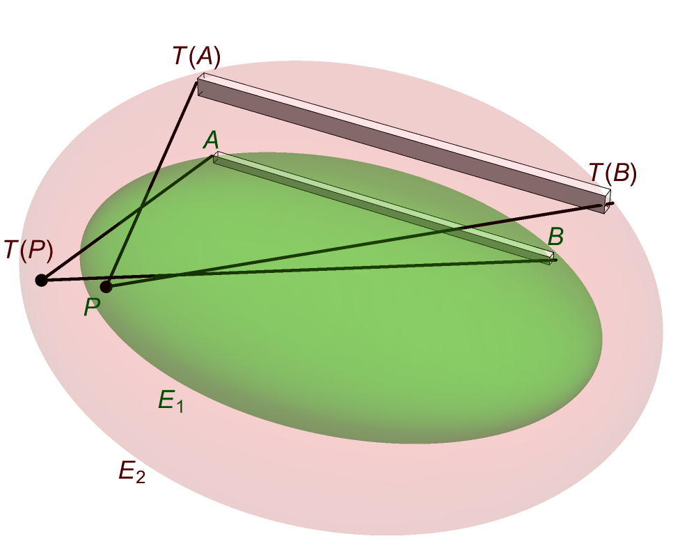
Given two ellipsoids, E1 and E2, with semi-axes ax, ay, az and αx, αy, αz, we can map points from the surface of E1 to the surface of E2 by rescaling each coordinate as follows:
T(x, y, z) = ((αx /ax) x, (αy /ay) y, (αz /az) z)
If E1 and E2 are confocal, then for μ = x, y, z we have:
(αμ/aμ)2 – 1
= (αμ2 – aμ2) / aμ2
= λ / aμ2
for some fixed λ that does not depend on the particular axis.
Let P = (px, py, pz) and Q = (qx, qy, qz) be any two points on the surface of E1.
dist(P, T(Q))2 – dist(T(P), Q)2
= Σμ [(pμ – (αμ/aμ) qμ)2 – ((αμ/aμ) pμ – qμ)2]
= Σμ [(qμ2 – pμ2) ((αμ/aμ)2 – 1)]
= λ Σμ [(qμ2 – pμ2) / aμ2]
= λ (Σμ [qμ2 / aμ2] – Σμ [pμ2 / aμ2])
= λ (1 – 1)
= 0
So dist(P, T(Q)) = dist(T(P), Q).
Another result we will need is that for a rod of uniform density, the component of the gravitational attraction of the rod, along the direction of the rod itself, at some point P, is proportional to the difference of the reciprocals of the distances of P from the endpoints of the rod, A and B. If we suppose the rod lies along the x-axis with endpoints at xA and xB and has cross-sectional area σ, while P lies at (0, d, 0), we have:
gx = G ρ σ ∫xAxB x / (d2 + x2)3/2 dx
= G ρ σ [1/(d2 + xA2)½ – 1/(d2 + xB2)½]
= G ρ σ [1/dist(P, A) – 1/dist(P, B)]
Now, consider two confocal ellipsoids, E1 and E2, with points P on the first and T(P) on the second, where T is the map between ellipsoids we defined previously. Let E1 be the smaller of the two ellipsoids. First, suppose that E1 is a solid ellipsoid of uniform density ρ, and we compute the gravitational attraction g(E1, T(P)) it exerts at the exterior point T(P). The point T(P) lies on E2, but here E2 is just a geometric construct to aid our calculations, containing no material. Then suppose we swap the roles of the ellipsoids, with E2 the solid ellipsoid of uniform density ρ, and we compute the gravitational attraction g(E2, P) it exerts at the interior point P, which lies on E1, which now is just an aid to the calculations.
It turns out that g(E1, T(P)) and g(E2, P) have a very simple relationship, and this will allow us to use what we know about g for interior points to find its value for exterior points.
We can compute the x-component of g(E1, T(P)) by breaking up E1 into infinitesimal rectangular rods aligned with the x-axis, running the full length of the ellipsoid, with cross-sectional area dy dz. If we call the endpoints of the rod A and B, our formula for a rod gives us:
dgx(E1, T(P))
= G ρ dy dz [1/dist(T(P), A) – 1/dist(T(P), B)]
Similarly, we can compute the x-component of g(E2, P) by breaking up E2 into a matching set of rods with endpoints at T(A) and T(B) and a suitably rescaled cross-sectional area (αy αz)/(ay az) dy dz.
dgx(E2, P)
= G ρ (αy αz)/(ay az) dy dz [1/dist(P, T(A)) – 1/dist(P, T(B))]
= G ρ (αy αz)/(ay az) dy dz [1/dist(T(P), A) – 1/dist(T(P), B)]
= (αy αz)/(ay az) dgx(E1, T(P))
So for every such rod, the two quantities are related by the same factor, which is independent of the choice of rod, and when we integrate over all rods to get the totals they will be related in exactly the same way. What’s more, we get analogous relationships for the other coordinate directions.
gx(E2, P) = (αy αz)/(ay az) gx(E1, T(P))
gy(E2, P) = (αx αz)/(ax az) gy(E1, T(P))
gz(E2, P) = (αx αy)/(ax ay) gz(E1, T(P))
Since P is an interior point of the larger ellipsoid, E2, we already know the acceleration due to gravity here:
g(E2, P) = –4 π G ρ (Aα px, Bα py, Cα pz)
We have written these coefficients as Aα, Bα, Cα to emphasise that they need to be computed with the semi-axes of E2.
This lets us write the acceleration due to gravity from E1 at the exterior point T(P):
g(E1, T(P)) = –4 π G ρ [(ax ay az) / (αx αy αz)] (Aα T(P)x, Bα T(P)y, Cα T(P)z)
The effect of choosing a specific ellipsoid E1 here is less that it might seem. E1 singles out a family of confocal ellipsoids, but any other member of that family would do the same. Other than that, its semi-axes only appear as the product ax ay az, which is proportional to its volume, V = (4/3) π ax ay az, so we could remove this by specifying the mass of the ellipsoid, M, rather than its density and dimensions. The function T is defined with respect to E1 and E2, but T(P) could be any exterior point and we no longer need to relate it to P.
Acceleration due to gravity exterior to an ellipsoid E with uniform density and mass M
g(E, (x, y, z)) = [–3 M G / (αx αy αz)] (Aα x, Bα y, Cα z)
αx, αy and αz are the semi-axes of an ellipsoid confocal with E such that (x, y, z) lies on its surface.
The coefficients Aα, Bα, Cα are those described previously for the interior potential, computed with these α semi-axes.
So, for any of the members of a family of confocal ellipsoids with uniform density, the gravitational field, g, at a given exterior point will differ only in proportion to the mass of the ellipsoid.
As a consistency check, note that for a sphere A = B = C = ⅓, and αx = αy = αz = r, so the formula above becomes:
g(S, (x, y, z)) = [–M G / r3] (x, y, z)
which is just the inverse-square law, as expected. Also, if we choose a point on the boundary of the ellipsoid, the α semi-axes will be equal to the semi-axes of the ellipsoid itself, and the formula above will agree with the one for the interior.
What about the potential? Since the acceleration g at a given exterior point for different confocal ellipsoids only differs in proportion to their mass, the same must be true of the potential (given the constraint that it always goes to zero at infinity), so we can compute the potential by finding the value it would have if the ellipsoid was enlarged until its boundary contained the point in question, while its density was reduced in order to keep its mass unchanged.
Potential exterior to an ellipsoid E with uniform density and mass M
Ψ(E, (x, y, z)) = [(3/2) M G / (αx αy αz)] (Aα x2 + Bα y2 + Cα z2 + Dα)
αx, αy and αz are the semi-axes of an ellipsoid confocal with E such that (x, y, z) lies on its surface.
The coefficients Aα, Bα, Cα, Dα are those described previously for the interior potential, computed with these α semi-axes.
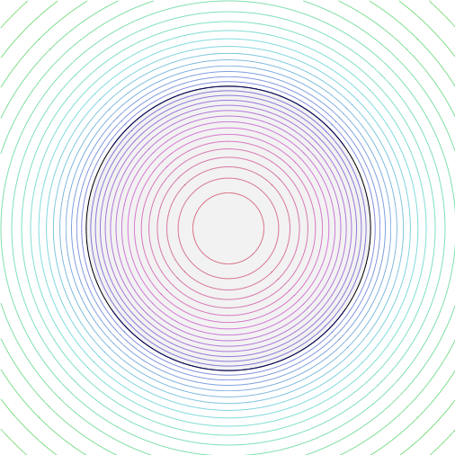
The image on the left shows a slice through the surfaces of equal potential for a range of ellipsoids of revolution, all with the same density and volume. The axis of symmetry is vertical in this image, and the semi-axes vary from √2, √2, 1/2 (the most oblate) to √[2/3], √[2/3], 3/2 (the most prolate).
The curves of equal potential are perfect ellipses in the interior, but those in the exterior are not. It is only in the case of a sphere that the entire surface of the body has equal potential, and would be experienced as gravitationally level. For a prolate spheroid, where the polar axis is longer, the poles lie “uphill” from the equator, while for an oblate spheroid the equator is “uphill” from the poles. In both cases, the acceleration due to gravity, g, is weakest at the point that is farthest from the centre.
So far, we have considered only non-rotating bodies, which maintain their ellipsoidal shapes through the strength of the materials from which they are composed, which are assumed to be non-deformable solids. This is possible for small enough objects, but beyond a certain size the pressure due to gravity will be sufficient to make most materials flow, and so non-rotating bodies will take on a spherical shape.
What about rotating bodies? If a body undergoes uniform rotation with an angular velocity of ω around the z-axis, that adds a “centrifugal potential” of:
Ψcen(x, y, z) = –½ω2(x2 + y2)
to the gravitational potential. The opposite of the gradient of this potential is:
acen = –∇Ψcen = ω2 (x, y, 0)
|acen| = ω2 r
which is the centrifugal acceleration that material instantaneously at rest in the rotating frame will undergo, if subject to no other force.
If we combine this potential Ψcen with the gravitational potential in the interior of an oblate spheroid, then the surfaces with a constant potential of Ψs will themselves be spheroids, satisfying the equation:
(2 π G ρ A – ½ω2)(x2 + y2) + 2 π G ρ C z2 + D = Ψs
For a body composed of fluid to be in equilibrium, the sum of gravitational and centrifugal force at its surface must be orthogonal to the surface. This means the surfaces of constant gravitational-plus-centrifugal potential must be the same shape as the body itself. The particular value of Ψs that the potential takes on at the surface of the body is not important, because all surfaces of constant potential will be the same shape apart from their overall scale. To match this shape with that of the body, an oblate spheroid with semi-axes a, a and c, we need:
(2 π G ρ A – ½ω2) a2 = 2 π G ρ C c2
ω2 / (π G ρ)
= 4 (A – (c2/a2) C)
= 2c (a2 + 2c2) acos(c/a) / (a2 – c2)3/2 – 6c2 / (a2 – c2)
It is common practice to express this result in terms of the eccentricity e of the meridians of the spheroid. An ellipsoid in this configuration is known as a Maclaurin spheroid, as this problem was solved by the mathematician Colin Maclaurin in 1742.
Squared angular velocity of a Maclaurin spheroid with semi-axes a, a and c,
eccentricity e = √[1 – c2/a2]
WMac(e) = ω2 / (π G ρ) = 2 (3 – 2e2) √[1 – e2] asin(e) / e3 – 6 (1 – e2) / e2
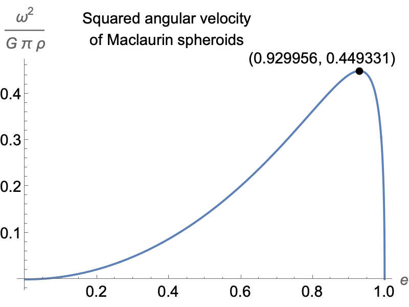
The squared angular velocity needed for equilibrium reaches a maximum of 0.449331 π G ρ at an eccentricity of 0.929956, after which it rapidly declines.
Note, though, that because the ellipsoid is becoming increasingly oblate — with a larger proportion of its mass lying further from the axis of rotation — a given quantity of material that changes its shape in this way will have an increasing moment of inertia. It turns out that even when the angular velocity that is required to maintain the shape begins to fall, the angular momentum will continue to increase. We will go into this in more detail shortly.
It is not possible to make the surface of a prolate spheroid an equipotential surface by spinning it around its axis. However, it can be done for an ellipsoid with three different semi-axes, a > b > c, spinning around the shortest axis, if a, b, c satisfy a further condition. In order for the meridians of the ellipsoid in both the xz and yz planes to match the shape of the meridians of the equipotential ellipsoids for the gravitational-plus-centrifugal potential, we must have:
ω2 / (π G ρ) = 4 (A – (c2/a2) C) = 4 (B – (c2/b2) C)
So A – B + c2 (1/b2 – 1/a2) C = 0
Define χ(a, b, c) = a2 b2 (B – A) / (a2 – b2) – C c2
Condition on semi-axes is χ(a, b, c) = 0
An ellipsoid meeting these conditions is known as a Jacobi ellipsoid, having been studied by the German mathematician Carl Gustav Jacob Jacobi.
Making use of the symmetrical form of the coefficients, we have:
Squared angular velocity of a Jacobi ellipsoid with semi-axes a, b, c,
rotating around c-axis.
WJac(a, b, c)
= ω2 / (π G ρ)
= 4 (A(a, b, c) a2 – B(a, b, c) b2) / (a2 – b2)
= 2 a b c ∫0∞ u du / ((a2 + u) (b2 + u) Δ)
Condition on semi-axes:
χ(a, b, c) = a2 b2 (B(a, b, c) – A(a, b, c)) / (a2 – b2) – C(a, b, c) c2 = 0
a2 b2 ∫0∞ du / ((a2 + u) (b2 + u) Δ) = c2 ∫0∞ du / ((c2 + u) Δ)
where Δ = √[(a2 + u)(b2 + u)(c2 + u)]

The plot on the left shows the value of χ(a, b, c), the function of the semi-axes that needs to be zero, for a range of b/a and for various values of the eccentricity exz of the xz meridians, where c/a = √[1 – exz2]. The hollow circles show the points on each curve where b = c, making it easier to see that the filled circles where each curve crosses the axis has b > c.

In order for the condition to be met with b ≤ a, the eccentricity exz must be greater than or equal to the critical value ecrit ≈ 0.812670 at which it is met for b/a = 1. But as the plot on the right shows, if exz < ecrit, although a solution can be found with b > a, the eccentricity of the meridians in the yz plane will satisfy eyz > ecrit. So every Jacobi ellipsoid must have the eccentricity of one of its vertex meridians greater than or equal to ecrit, and the other less than or equal to ecrit.

The plot on the left compares the squared angular velocity for the Maclaurin spheroids (red curve) and Jacobi ellipsoids (green and blue curves), as a function of the eccentricity of the xz meridian. The green curve, where exz ≤ ecrit, does not describe a separate family of ellipsoids from the blue curve, where exz ≥ ecrit, because we can transform one into the other just by changing the way we label the x and y axes for the ellipsoid.
At the critical eccentricity, the Jacobi ellipsoid is simply a Maclaurin spheroid. But for other values, we can ask whether a given mass of fluid rotating as a Maclaurin spheroid would have a higher or lower total energy if it took the form of Jacobi ellipsoid instead.
To characterise the body of fluid we are dealing with, we will follow Chandrasekhar in using the total mass M and the geometric mean of the three semi-axes:
a̅ = (a b c)⅓
This fixes the volume at:
V = (4π/3) a̅3
and corresponds to a density of:
ρ = M / V = 3M / (4π a̅3)
For a spheroid with semi-axes a, a, c = a √[1 – e2], we have:
a / a̅ = 1 / (1 – e2)1/6
We will make the comparison between the Maclaurin spheroid and Jacobi ellipsoid forms that a given body of fluid can take for the same value of angular momentum. The angular momentum of an isolated body is conserved even as it changes shape, whereas angular velocity will vary as the moments of inertia of the body change.
The inertia tensor Iij of a homogeneous ellipsoid can be found from the second-order moments Jij, which we previously calculated:
J11 = (M/5) a2
J22 = (M/5) b2
J33 = (M/5) c2
Iij = δij tr(J) – Jij
I11 = (M/5) (b2 + c2)
I22 = (M/5) (a2 + c2)
I33 = (M/5) (a2 + b2)
with all non-diagonal elements zero. The inertia tensor lets us compute both the angular momentum and the kinetic energy of a rotating ellipsoid, given its angular velocity. While the angular velocity and the angular momentum are both vectors, we are focusing on the specific scenario where the ellipsoid is rotating around the z-axis, so in what follows both the angular velocity ω and the angular momentum L will refer to the z-component of the vectors, with the other components zero.
With that understood, we have for the angular momentum L and the rotational kinetic energy K:
L = I33 ω
K = ½ I33 ω2
What about the potential energy of the fluid, due to its own gravitational attraction?
U = ½ ∫ Ψ(x, y, z) ρ dV
= π G ρ ∫ (A x2 + B y2 + C z2 + D) ρ dV
= π G ρ (A J11 + B J22 + C J33 + M D)
= π G ρ M [(1/5)(A a2 + B b2 + C c2) + D]
But as we previously found (and can easily verify using the formulas for the coefficients):
A a2 + B b2 + C c2 = –D
This gives us:
U = (4/5) π G ρ M D
= (3/5) G M2 D / a̅3
or equivalently:
U = (2/5) M Ψ0
where Ψ0 is the potential at the centre of the ellipsoid.
For the Maclaurin spheroid, where a = b, the angular momentum as a function of the eccentricity of the meridians can be written as:
LMac = I33 ω = (2/5) M a2 √[(π G ρ) WMac(e)]
LMac / √[G M3 a̅] = (√3)/5 √[WMac(e)] / (1 – e2)⅓
We do not have a closed form expression for the Jacobi case, but we can express it in equivalent terms as:
LJac / √[G M3 a̅] = (√3)/10 √[WJac(a(exz), b(exz), c(exz))] (a(exz)2 + b(exz)2) / a̅(exz)2
with the understanding that we find the value of eyz that meets the Jacobi condition for a given exz, which then gives us the ratios between the semi-axes that we need to compute WJac(a(exz), b(exz), c(exz)) and the ratios of the semi-axes to a̅.

The plot on the left compares the angular momentum for the Maclaurin spheroids (red curve) and Jacobi ellipsoids (green and blue curves), as a function of the eccentricity of the xz meridian.
Note that there is a minimum angular momentum for a given body of fluid below which it cannot form a Jacobi ellipsoid. This value, LJac, min ≈ 0.303751, is measured in units of √[G M3 a̅], which are specific to the body’s mass and volume.
 |
 |
 |
 |
We will use the relationship between the angular momentum and the eccentricities of the Maclaurin spheroids and Jacobi ellipsoids to map L back to exz (for the Jacobi ellipsoids we can simply choose the higher eccentricity, as the two eccentricities are not independent). We can then use formulas for the kinetic and potential energy as functions of the eccentricity to determine their relationship to the angular momentum for the Maclaurin and Jacobi forms the body can take.
From the plot on the right it can be seen that the eccentricity of the xz meridian at a given angular momentum for the Jacobi ellipsoid (blue curve) is initially greater than for the Maclaurin spheroid (red curve), starting from LJac, min, then eventually becomes slightly less, for L / √[G M3 a̅] > 0.681126. This does not mean that the overall shape of the two forms becomes the same again when these curves intersect; since this value for exz is greater than ecrit, the value of eyz for the Jacobi ellipsoid will be lower than ecrit.
The kinetic energy of a Maclaurin spheroid is:
KMac = ½I33 ω2 = (1/5) M a2 (π G ρ) WMac(e)
KMac / (G M2 / a̅) = (3/20) WMac(e) / (1 – e2)⅓
The potential energy of a Maclaurin spheroid is:
UMac = (3/5) G M2 D / a̅3
= –(3/5) (G M2 / a̅) (a / a̅)2 c acos(c/a) / √[a2–c2]
= –(3/5) (G M2 / a̅) √[1 – e2] / (1 – e2)⅓ asin(e) / e
UMac / (G M2 / a̅) = –(3/5) (1 – e2)1/6 asin(e) / e
The equivalent formulas for the Jacobi ellipsoid are:
KJac / (G M2 / a̅) = (3/40) WJac(a(exz), b(exz), c(exz)) (a(exz)2 + b(exz)2) / a̅(exz)2
UJac / (G M2 / a̅) = (3/5) D(a(exz), b(exz), c(exz)) / a̅(exz)2
The plots on the right show that the relationship between the kinetic and potential energy of the two forms and the angular momentum is quite complicated, with the Maclaurin and Jacobi curves crossing after they initially part at LJac, min. But the total energy ends up consistently less for the Jacobi ellipsoids, for the physically relevant range.
What this means is that if a spinning body of fluid has an angular momentum greater than LJac, min and it is in the form of a Maclaurin spheroid, then if it is able to lose energy (without changing its angular momentum or shedding mass) it will evolve into the Jacobi form. For example, a viscous fluid might be able to convert some of its kinetic energy of rotation into heat. The details of viscous dissipation are beyond the scope of this web page, but are covered in Chandrasekhar.[3]
The instability of the Maclaurin spheroids with respect to the lower energy of the Jacobi ellipsoids is known as secular instability. At higher angular momentum, both kinds of body are also subject to dynamic instability, whereby small changes in their shape will grow exponentially (rather than leading to small oscillations). For the Maclaurin spheroids, this occurs at:
e ≈ 0.952887
ω2 / (π G ρ) ≈ 0.440220
LMac / √[G M3 a̅] ≈ 0.509119
For the Jacobi ellipsoids it occurs at:
exz ≈ 0.938577
eyz ≈ 0.602206
ω2 / (π G ρ) ≈ 0.284031
LJac / √[G M3 a̅] ≈ 0.389536
The details can be found in Chandrasekhar.[4]
 |
 |
The images on the left show the gravitational-plus-centrifugal equipotential surfaces for two ellipsoids with different shapes, but the same mass and volume, as they increase their angular velocity until both have the same angular momentum. The first is a Maclaurin spheroid, the second a Jacobi ellipsoid.
The ellipsoids here are treated as solid bodies with enough material strength to retain a fixed shape regardless of their motion, purely for the sake of illustrating how the shapes of the equipotential surfaces change, becoming identical to that of the bodies themselves once the final angular momentum is reached.
The potential energy, U, of the Maclaurin spheroid is slightly lower than that of the Jacobi ellipsoid, but the Jacobi ellipsoid, with its greater moment of inertia I, reaches the same angular momentum, L, with a smaller angular velocity ω, and ends up with a kinetic energy, K, that is smaller by a sufficient margin to make its total energy, E, the lower of the two.
[For these examples we have set G = M = a̅ = 1, so the angular momentum units √[G M3 a̅] and the energy units G M2 / a̅ are both equal to 1. However, this makes the squared angular velocity units π G ρ equal to 3/4, so the values of ω shown here need to be squared and multiplied by 4/3 to yield values for ω2 / (π G ρ), which turn out to be 0.4323 for the Maclaurin spheroid and 0.2927 for the Jacobi ellipsoid.]
Because the total (gravitational-plus-centrifugal) potential is the same at all the vertices of these ellipsoids, the ratio between the total acceleration at any two vertices is just the inverse ratio of the semi-axes. For example:
Ψtotal, a = Ψtotal, b
(2 π G ρ A – ½ ω2) a2 = (2 π G ρ B – ½ ω2) b2
–½gtotal, a a = –½gtotal, b b
gtotal, a / gtotal, b = b / a

The image on the right shows a body of fluid with the same mass and volume as the previous examples, adopting the minimum energy configuration as its angular momentum increases and decreases.
[1] Ellipsoidal Figures of Equilibrium, S. Chandrasekhar. Revised edition, Dover, New York, 1987.
[2] Chandrasekhar, op. cit. Chapter 1, Equation 7.
[3] Chandrasekhar, op. cit. Chapter 5, Section 37.
[4] Chandrasekhar, op. cit. Chapter 5, Equation 59, for the onset of dynamic instability in the Maclaurin spheroid, and Chapter 6, Equation 57, for the onset of dynamic instability in the Jacobi ellipsoid.
[5] The Mathematical Principles of Natural Philosophy, Isaac Newton. Translated from Latin into English by Andrew Motte. Published by Daniel Adee, New York, 1846. Available through Project Gutenberg at https://www.gutenberg.org/files/76404/76404-h/76404-h.htm. BOOK III. PROPOSITION XIX. PROBLEM III.
[6] Newton, op. cit. BOOK I. PROPOSITION XCI. PROBLEM XLV. COR 2.
[7] “The optimal shape of an object for generating maximum gravity field at a given point in space”, Xiao-Wei Wang and Yue Su. Eur. J. Phys. 36 (2015) 055010. Online at https://arxiv.org/abs/1412.5541.