
The image above shows a body moving under an inverse-square law of attraction, like a planet around a star. The blue vector v is its velocity. The vector er is a unit-length vector that rotates to follow the body around its orbit, while eθ is a unit-length vector perpendicular to er. The green vector is equal to eθ multiplied by a factor of k/L, where k is the acceleration constant in the inverse-square force law, and L is the angular momentum of the body per unit mass, which is a constant for any particular orbit.
The red vector, which we will call S, is the difference:
S = (k/L) eθ – v
You will notice that S seems to be a constant vector, never changing its size or direction. We can easily prove that this is the case. First, note that because of the conservation of angular momentum, the angular velocity of the body around the centre is:
ω = L/r2
where r is the distance from the centre of attraction to the body. It follows that the rate of change of eθ with time is:
deθ/dt = –ω er = –(L/r2) er
What is the rate of change of the velocity, v, with time? Since the body is subject to an inverse-square force law, and we have said that the relevant acceleration constant is k, we have:
dv/dt = –(k/r2) er
So, we have two vectors whose rates of change both follow inverse-square rules, and are multiples of er. We chose S to be a linear combination of these vectors whose rate of change cancels out to zero:
dS/dt = (k/L) deθ/dt – dv/dt = 0
Now, the relationship between angular velocity ω, angular momentum per unit mass L, and distance r will hold true for any central force: any force that is directed towards a fixed point of attraction. This will always yield an inverse-square rule, ω = L/r2. So what is special here is that we have chosen a particular central force (like gravity, or electrostatic attraction) where the acceleration also obeys an inverse-square rule. That is why we can define this constant vector S; it is a special consequence of an inverse-square force law.
I learned about this vector S from a tweet by Albert Chern, but it is intimately related to a famous conserved vector known as the Laplace-Runge-Lenz (LRL) vector. The latter is much more widely known – but as we have just seen, the fact that S is conserved for any inverse-square force law is ridiculously easy to prove, whereas most proofs that the LRL vector is conserved are much longer, and the reason they hold true is not as transparent.
How are the two related? The LRL vector, A, can be defined as:
A = m2 (v × L – k er)
where m is the mass of the body, and L is the angular momentum vector of the body, per unit mass. L is perpendicular to the plane of the orbit. (The definitions you find elsewhere might differ by an overall factor of m, and may also use a version of L that is the full angular momentum, rather than the angular momentum per unit mass, and a version of k that gives the force on the orbiting body rather than the acceleration.)
This can be constructed from S as follows:
m2 L × S = m2 L × ((k/L) eθ – v)
= m2 (v × L – k er)
= A
So, along with the fact that L is a constant vector perpendicular to the plane of the orbit, and S is a constant vector that lies in the plane of the orbit, this simple calculation is enough to prove that the LRL vector A must be a constant vector that lies in the plane of the orbit and is perpendicular to S.
What is the direction of A? When the orbit crosses the major axis of the ellipse, both v and eθ will be perpendicular to that axis, so S must (then, and always) be perpendicular to it, and A (then, and always) will be parallel to it.
What about the magnitude of A? Suppose the body has minimum and maximum distances from the centre of attraction of r1 and r2. These will occur when it lies on the major axis of the ellipse, where the velocity will be parallel to eθ, and where we have:
v = L/r
Equating the value of S at these two points (and using eθ(θ=0) = –eθ(θ=π)) gives us:
k/L – L/r2 = –(k/L – L/r1)
which we can solve to obtain:
L2 = 2 k r1 r2 / (r1 + r2)
If we substitute this into:
A = m2 L (k/L – L/r2)
= m2 (k – L2/r2)
we end up with:
A = m2 k (r2 – r1)/(r1 + r2)
= m2 k ε
where ε is the eccentricity of the orbit.
There is much, much more that can be said about the Laplace-Runge-Lenz vector; it comes up in discussions of the hidden 4-dimensional symmetries of the inverse-square law, and the reason orbits are conic sections. But here, we will look at just one more topic: how the Laplace-Runge-Lenz vector is derived using Noether’s Theorem.
[No, this section is not easy. The “LRL made easy” part was the simple proof at the start of this page that the Laplace-Runge-Lenz vector is conserved.]
There is a famous connection between conserved quantities in physical systems and a certain kind of symmetry that is encapsulated by Noether’s theorem. This theorem is phrased in the language of Lagrangian mechanics, but if you are not already familiar with that subject, you can find a quick overview here.
In Noether’s theorem, we start with the idea of taking a trajectory a particle follows and looking at what changes if we move every point on the trajectory in some systematic way. In the simplest examples, we might ask what happens if we translate the whole trajectory by a constant amount in a certain direction, or if we rotate the whole trajectory about some axis. The fact that the Lagrangian for a free particle is left unchanged if we do either of those things allows us to prove, via Noether’s theorem, that a free particle has conserved momentum and angular momentum vectors.
Noether’s theorem also applies if we perform more elaborate operations on the trajectory. We can move points on the trajectory by an amount that depends on their position (as happens for a rotation), but also on the velocity of the trajectory at that point. (There are other possibilities too, but that is all we will need for our current purposes.) The simplest way to talk about these changes is to write down a formula for a vector in ordinary space that gives the direction in which we wish to move points on the trajectory. The formula that will be of interest to us actually gives us three different vectors at once, where we make a specific choice by setting s equal to x, y or z:
X(s) = ½ (2 xs v – vs x – (x · v) es)
Here, the terms xs and vs refer to the x, y or z coordinates of the particle’s position or velocity, while es is a unit-length vector in one of the three coordinate directions.
For the simple examples we mentioned earlier, it would be easy to draw a vector field in space that showed, for each point, the direction we would be moving it. For a translation, we would just draw a whole lot of arrows of equal length pointing in the same direction. For a rotation, we would draw arrows pointing in circles around the axis, whose length was proportional to their distance from the axis. But our X(s) vectors depend on the velocity of the particle, so we can’t just draw a vector at a point; we would need to go to the 6-dimensional space that includes both 3 coordinates in space and 3 velocity coordinates. What’s more, although we are only explicitly specifying how points on the trajectory should be moved in space, as a result of the way the vector changes from point to point, we are also changing the velocities along the trajectory, in a way that will depend both on the velocity and the acceleration.
So, we won’t try to draw a picture of X(s) directly. However, once we have examined the way it alters a few quantities associated with the particle, we will be in a better position to visualise its effects.
How does some some quantity, say f, that is a function of both the coordinates and velocity of the particle, change when we displace the particle, all along its trajectory, by an amount that depends on X(s)? We encapsulate this as a kind of directional derivative that gives us the instantaneous rate of change of f as a result of such a displacement:
X(s)(f) = X(s) · ∇x f + Σj (vj ∂X(s)/∂xj + aj ∂X(s)/∂vj) · ∇v f
where aj is the j component of the particle’s acceleration, Σj means “take the sum for j = x, y and z,” and:
∇x f = (∂f/∂x1, ∂f/∂x2, ∂f/∂x3)
∇v f = (∂f/∂v1, ∂f/∂v2, ∂f/∂v3)
This looks quite complicated, but the first term is just an ordinary directional derivative, where we take the dot product between the vector giving the direction we are moving along and the gradient of the function f, while the second term accounts for the change in the velocity of the particle, which comes from the fact that we are not just shifting the trajectory uniformly, we are potentially changing its shape and orientation.
Why are the partial derivatives of X(s) with respect to the coordinates and velocities multiplied by the components of the particle’s own velocity and acceleration? If the particle happened to have, say, vx = 0, then the fact that X(s) changed with x would make no difference, since x itself would not be changing for the particle, and following X(s) would, in that case, be a constant shift in the x direction that left vx unchanged. Similarly, if the particle happened to have ax = 0, the fact that X(s) changed with vx would make no difference. But by multiplying these partial derivatives by the current velocity and acceleration, and summing over all coordinate indices j, we arrive at the overall rate of change in the velocity due to following X(s), which then feeds into the change in f by taking the dot product with the gradient of f with respect to velocity coordinates.
To apply this formula, we are going to need the partial derivatives of X(s):
∂X(s)/∂xj = ½ ∂/∂xj (2 xs v – vs x – (x · v) es)
= ½ (2 δsj v – vs ej – vj es)
∂X(s)/∂vj = ½ ∂/∂vj (2 xs v – vs x – (x · v) es)
= ½ (2 xs ej – δsj x – xj es)
Here δsj is the Kronecker delta, equal to 1 if s = j, and 0 otherwise.
We will now compute the rates of change of some quantities associated with a particle subject to an inverse-square acceleration, starting with its kinetic energy per unit mass:
K = ½ v2 = ½ (vx2 + vy2 + vz2)
∂K/∂xj = 0, so ∇x K = 0
∂K/∂vj = vj, so ∇v K = v
X(s)(K) = Σj (vj ∂X(s)/∂xj + aj ∂X(s)/∂vj) · v
= ½ Σj (vj (2 δsj v – vs ej – vj es) – (k/r3) xj (2 xs ej – δsj x – xj es)) · v
= ½ (2 vs v2 – vs v2 – vs v2 – (k/r3) (2 xs (x · v) – xs (x · v) – vs r2)
= –k/(2r3) (xs (x · v) – vs r2)
and its potential energy per unit mass:
U = –k/r
∂U/∂xj = k xj /r3, so ∇x U = k x/r3
∂U/∂vj = 0, so ∇v U = 0
X(s)(U) = X(s) · ∇x K
= ½ (2 xs v – vs x – (x · v) es) · k x/r3
= k/(2r3) (xs (x · v) – vs r2)
We immediately have the nice result that for the total energy per unit mass:
E = K + U
X(s)(E) = X(s)(K) + X(s)(U)
= 0
Just as easily, if not quite as nicely, we have for the Lagrangian:
ℒ = m (K – U)
X(s)(ℒ ) = m (X(s)(K) – X(s)(U))
= mk/r3 (vs r2 – xs (x · v))
That shifting the trajectory with X(s) preserves the total energy, but not the Lagrangian, might seem like a mistake at first. Doesn’t Noether’s theorem apply to symmetries of the Lagrangian? In fact, what Noether’s theorem tells us is that:
d/dt (p · X(s)) = X(s)(ℒ )
where p is the Hamiltonian momentum, which in this case is simply p = mv.
If we had X(s)(ℒ ) = 0, then the identity above would instantly tells us that the quantity whose time derivative appears on the left hand side was conserved. But even though that isn’t the case, all is not lost. We have:
d/dt (xs / r) = d/dt (xs / √(x · x))
= vs / r – xs (x · v) / r3
= 1/r3 (vs r2 – xs (x · v))
It follows that:
d/dt (p · X(s) – mk xs / r) = X(s)(ℒ ) – mk/r3 (vs r2 – xs (x · v))
= 0
Now, the LHS really does represent the rate of change of a conserved quantity! And if we work through the details, we find:
p · X(s) – mk xs / r
= ½ mv · (2 xs v – vs x – (x · v) es) – mk xs / r
= m (xs (v · v) – vs (x · v)) – mk xs / r
= m es · (v × (x × v) – k er)
= m es · (v × L – k er)
= es · A / m
That is, the conserved quantities we have derived from our three vectors, X(s), are essentially the three components of the Laplace-Runge-Lenz vector.
Now, the proof at the start of this page gives a much shorter and more transparent way to see why the Laplace-Runge-Lenz vector is conserved. But our real aim here is to get a better understanding of how the vectors X(s) change the trajectory. We won’t work through all the details of the calculations, but using the same method as we applied to the kinetic and potential energy, we can show that:
X(s)(L) = ½ es × A / m2
X(s)(A) = –E m2 es × L
Let’s choose a coordinate system where the origin lies at the centre of attraction, the x axis runs along the major axis of the elliptical trajectory, and the y axis runs along the minor axis. Then the angular momentum vector, L, perpendicular to the plane of the orbit, will be a multiple of ez, and the LRL vector A will be a multiple of ex.
With those choices, we have for s = z:
X(z)(L) = ½ A / m2 ez × ex = ½ A / m2 ey
X(z)(A) = –E m2 L ez × ez = 0
A is unchanged, and the change in L is perpendicular to L, so X(z) acts to rotate the orbit around its major axis, taking it out of its original plane.
For s = x:
X(x)(L) = ½ A / m2 ex × ex = 0
X(x)(A) = –E m2 L ex × ez = E m2 L ey
L is unchanged, and the change in A is perpendicular to A, so X(x) acts to rotate the orbit around L, i.e. within its original plane.
For s = y:
X(y)(L) = ½ A / m2 ey × ex = –½ A / m2 ez
X(y)(A) = –E m2 L ey × ez = –E m2 L ex
Both vectors undergo changes parallel to themselves, so they retain their direction but change their magnitude. This means that X(y) acts to change the shape of the orbit, without affecting its orientation. If we continue to apply this change, with a parameter λ measuring how far we have proceeded, we can treat this as a pair of coupled ordinary differential equations for L(λ), the z component of the angular momentum, and A(λ), the x component of the Laplace-Runge-Lenz vector:
L'(λ) = –1/(2m2) A(λ)
A'(λ) = –E m2 L(λ)
This system will have sinusoidal solutions, with L(λ) having its maximum magnitude when A(λ) = 0, and vice versa.
We know that X(y) leaves the total energy of the particle constant, and that corresponds to preserving the length of the major axis of the elliptical orbit. So X(y) will just alter the length of the minor axis, which is proportional to the angular momentum. The image below shows an orbit changing under this flow; some individual points are shown as well.
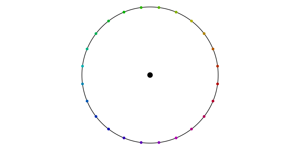
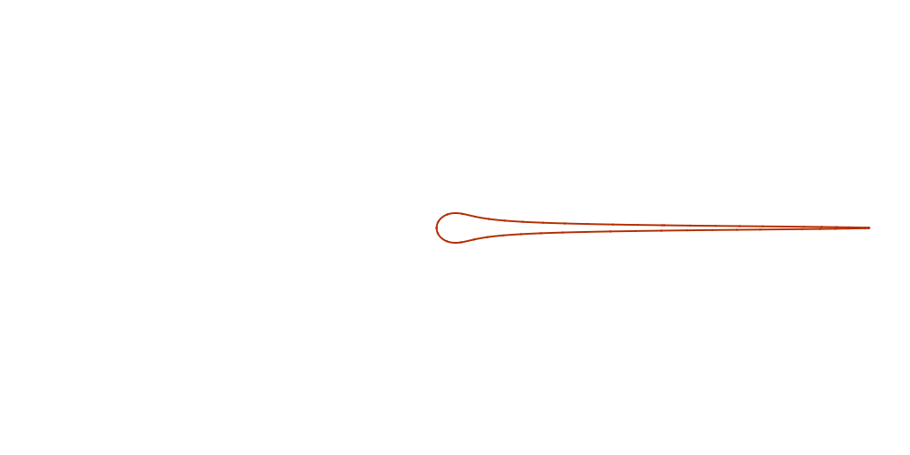
The individual points were tracked by solving the flow equations numerically, but they must also correspond to the locations on the different orbits reached at various fixed times. These are the curves that are traced out by each point:
As the orbit in space undergoes these changes, the curve traced out in the space of velocities will also change. These curves are always circles, but they will shift in size and position. In fact, they will correspond to the stereographic projections of a great circle rotating on a sphere in four dimensional-space! This is described in detail here.
