
What is the average area of the shadow cast by a cube, if we take the average over all possible orientations of the cube, while keeping its centre fixed?
This question was posed in a delightful video by Grant Sanderson, and answered for the case where the light source is infinitely far above the ground, so the shadow is cast by parallel rays. I won’t state the formula right now, so as not to spoil it if you decide to watch the video, or work out the answer for yourself. The derivation is a lot of fun, and you might find the result surprisingly simple.
On this page, we will find the average area of the shadow for the case where the light source is at a finite distance, but with the simplifying feature that it will be located directly above the centre of the cube.
We will assume that:
The quantity ½√3 here is the distance from the centre of the cube to one of its vertices, so the condition on δ will ensure that, however the cube is oriented, the light source is always outside the cube. We could impose a similar condition on h, so that no portion of the cube is ever below the ground, but although that would be necessary for the problem to make sense physically, all the geometry of rays from the light source intersecting the ground continues to work for any value of h.
What does it mean to take an average over all possible orientations of the cube? One way to formalise this is to suppose that we start with the cube in a certain orientation, then average over the result of applying all possible rotations. The group of all rotations in three dimensions, known as SO(3), can be given a coordinate system and a measure, which is essentially a probability distribution, assigning to each subset of the space a number such that the whole space has a measure of 1. What’s more, there is a unique way of doing this, such that the measure of a set of rotations is unchanged if we multiply them all by any other fixed rotation. In general, this is known as the Haar measure of the group. If, instead of the rotations themselves, we work with unit quaternions, the space we are considering will be the 3-dimensional surface of a hypersphere in four dimensions, and the Haar measure is the usual geometric measure of volume that the surface inherits from 4-dimensional Euclidean space.
If all of that sounds a bit abstract, don’t worry, because the consequences of formalising things this way are precisely what you would expect, intuitively. Any vector in our initial orientation of the cube (say, a vector n normal to one of the faces) ends up with equal probability of pointing in any direction, so we can average it over the 2-dimensional surface of an ordinary sphere in three dimensions. And any vector e that is orthogonal to n (say, the direction of an edge on the corresponding face of the cube) ends up having equal probability of pointing in any of the circle of directions orthogonal to n in its rotated position. So, if we sweep n over a sphere of directions, and e over a circle of directions orthogonal to n, we will have all orientations covered, with the correct probabilities.
We will proceed by computing the average area of the quadrilateral shadow cast on the ground by a single face of the cube, as the cube itself is swept through all possible orientations while its centre is kept fixed. The shadow of the whole cube is a more complicated polygon, but its area at any instant will be equal to half the sum of the areas of the shadows of all six faces, because each geometric ray casting the shadow will enter the cube on one face and leave it on another. Since all six faces must, by symmetry, have the same average area, the average area of the cube’s shadow will be exactly three times the average area of a single face’s shadow.
Suppose the outward-pointing normal vector to the face is:
n = (sin θ cos φ, sin θ sin φ, cos θ)
where θ measures the angle from the vertical, and ranges from 0 to π, while φ is a longitudinal angle ranging from 0 to 2π. If we integrate over these variables, we need to weight the quantity we are averaging by sin θ, the radius of a circle on the unit sphere at an angle of θ from the north pole, and then divide the integral by 4π, the total area of the unit sphere.
Given that direction for the face normal n, we will suppose that the two directions of the face edges are:
e1 = (–sin α cos θ cos φ – cos α sin φ, cos α cos φ – sin α cos θ sin φ, sin α sin θ)
e2 = (–cos α cos θ cos φ + sin α sin φ, –sin α cos φ – cos α cos θ sin φ, cos α sin θ)
These are unit vectors that are orthogonal to each other, and both are orthogonal to n, with α specifying the amount of rotation in the plane orthogonal to n. If we integrate the quantity we are averaging over α from 0 to 2π, we then need to divide by 2π.
The four vertices of the face are then given by:
v = (0,0,h) + ½n ± ½e1 ± ½e2
We project these vertices with rays from the light source, at s = (0,0,h+δ), to the ground:
P(x, y, z) = [(h+δ) / (h+δ–z)] (x, y)
The area of any triangle in two dimensions can be found as half the determinant of the 2×2 matrix whose columns are two edge vectors of the triangle (the angle moving counterclockwise from the first edge to the second must pass through the interior of the triangle to yield the correct sign). The area of any triangle in three dimensions can be found as half the magnitude of the cross product of any two edges. Combining these with our projection formula, with a bit of algebra it is not too hard to show that the factor by which the area of a triangle is multiplied to give the area of its shadow is:
Triangle shadow area factor = ½(h+δ)2 (n · (t – s)) / [(z1 – h – δ) (z2 – h – δ) (z3 – h – δ)]
Here zi are the z coordinates of the triangle’s vertices, n is a unit vector normal to the plane of the triangle, t can be any point at all in the plane of the triangle (we could pick one of the vertices to be concrete), and s = (0,0,h+δ) is the light source. This gives a positive factor overall if the vector n points from the triangle towards the light source; the three terms in the denominator are all negative, because the triangle must lie below the light source.
If we divide our square face into two triangles with equal area of ½, the area of the shadow of the face will just be the average of these factors for the two triangles. If we grind through all the calculations, we end up with:
A(θ, α) = | 4 (h + δ)2 (2δ – cos θ) (2δ cos θ – 1) / ((2δ – cos θ)4 – 2 (2δ – cos θ)2 sin2 θ + (cos2 α – sin2 α)2 sin4 θ) |
Note that the angle φ does not appear here at all! Because we have chosen to place the light source directly above the centre of the cube, the longitudinal angle makes no difference to the size of the shadow. As a further check that this formula makes sense, we can put θ=0, which gives:
A = 4 (h + δ)2 / (2δ – 1)2
Putting z=h+½ in the projection formula gives a linear scaling factor whose square matches this.
We will perform the integration over α first. Because α measures the rotation of the face in its own plane, the value of α cannot have any effect on the sign of the quantity we are using to compute the area. So we can integrate over the full range of α without worrying about having to take the opposite value of the integrand for part of the range (as we will need to do for θ).
We will make use of the formula:
1/(2π) ∫02π 1 / (b + (cos2 α – sin2 α)2) dα = 1 / √[b (b+1)]
This can be proved fairly easily by means of Cauchy’s residue theorem, after converting the denominator of the integrand into:
b + (cos2 α – sin2 α)2 = ½(1 + 2b + cos 4α)
This expression has four distinct zeroes with real parts between 0 and 2π in the upper half-plane of the complex numbers. By deforming the integral from 0 to 2π to loop around these four zeroes, the residues of the original function can be added up to give the result we are claiming.
This lets us average the area over α, obtaining:
A(θ) = | 4 (h + δ)2 (2 δ cos θ – 1) / [(2 cos2 θ – 4 δ cos θ + 4 δ2 – 1) √(3 cos2 θ – 4 δ cos θ + 4 δ2 – 2)] |
The sign of the quantity whose absolute value we are taking depends entirely on the (2δ cos θ – 1) term in the numerator. Neither of the expressions in the denominator have real zeroes for θ, given the restriction we have imposed on δ. So we can integrate the expression and its opposite over the two ranges for θ where the sign is constant, on either side of arccos(1/(2δ)).
When we integrate over θ, we need to multiply the expression above by sin θ to get the correct measure on the sphere of directions, and then divide by 2. Why 2, and not the area of the sphere, 4π? Because there is no dependence on φ, we aren’t going to bother explicitly integrating for φ from 0 to 2π, but if we did, that would introduce a factor of 2π, and then dividing by 4π would simply be the same as dividing by 2.
This integral can be performed after making the substitution u = cos θ. The indefinite integral can then be expressed as:
I(u) = (h + δ)2 arctan( ( (u – 2 δ) √(3 u2 – 4 δ u + 4 δ2 – 2)) / (u2 – 1) )
Or, in a form you can cut and paste into software like Mathematica, if you want to verify the derivative:
(d + h)^2*ArcTan[((-2*d + u)*Sqrt[-2 + 4*d^2 - 4*d*u + 3*u^2])/(-1 + u^2)]
Then the sum of the two definite integrals, with the appropriate signs, multiplied by half the number of faces, yields a final result:
Average unit cube shadow = 3 (h + δ)2 arctan( (√(3 – 16 δ2 + 16 δ4)) / (1 – 8 δ2 + 8 δ4) )
Some care is needed taking the arctan here; when the denominator crosses zero so the argument becomes negative, we need to choose the value of the angle that lies in the second quadrant (i.e. between π/2 and π) rather than using negative values.
These features are illustrated in the plot below. The numerical values here correspond to setting h=1.
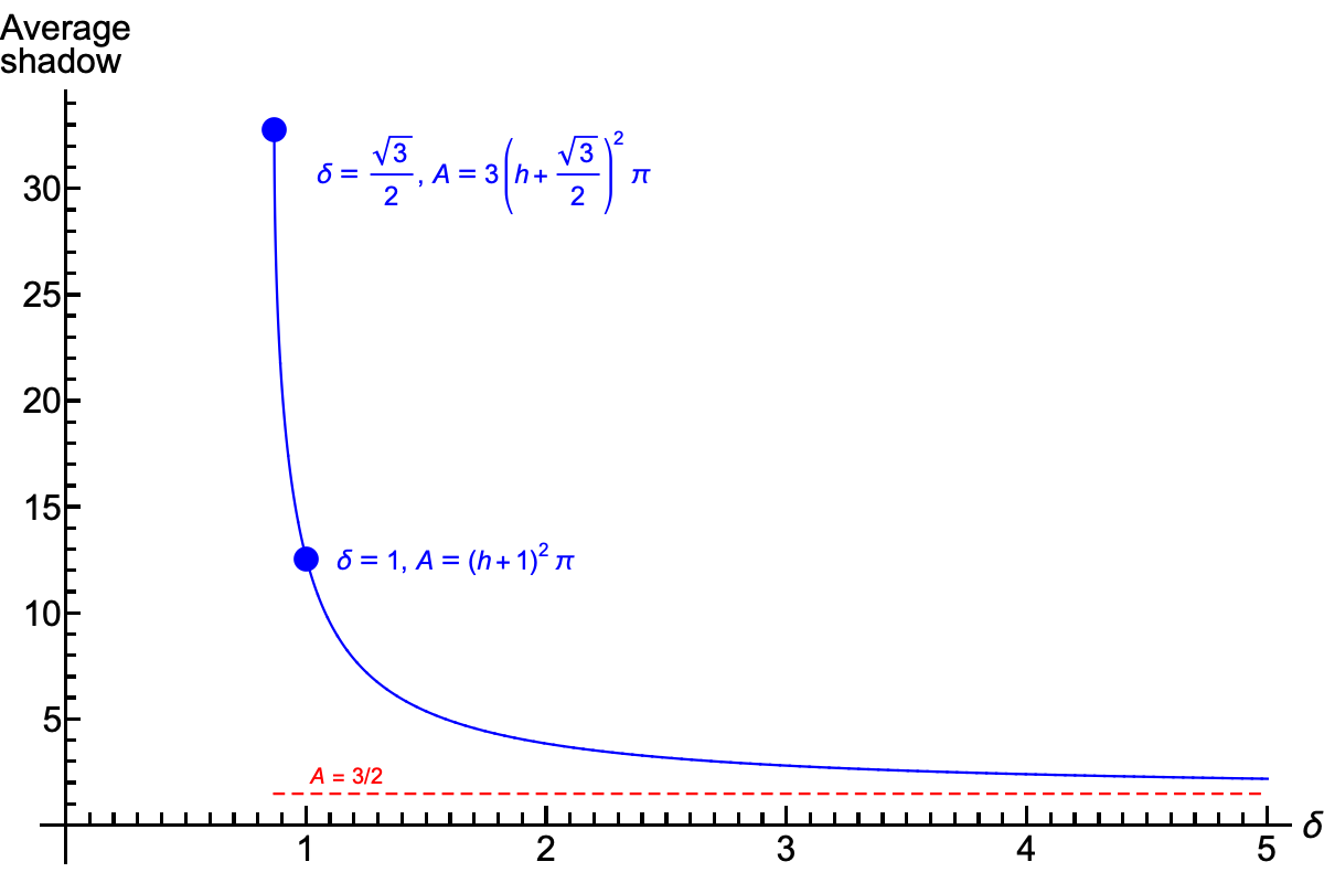
The average shadow area for a cube with any edge length can be found by rescaling the unit cube version:
Average cube shadow, edge length L = 3 (h + δ)2 arctan( L2 (√(3L4 – 16 δ2 L2 + 16 δ4)) / (L4 – 8 δ2 L2 + 8 δ4) )
We could generalise these calculations to any convex polyhedron at all, but to keep the results simple we will impose the restriction that all the faces are regular polygons, with the line from the centre of the face to the centre of the polyhedron perpendicular to the plane of the face. That includes the Platonic solids, whose faces are identical regular polygons, but we won’t need to assume that all the faces are the same, as different sets of faces can always be averaged separately then added together.
Consider a face that is a regular m-gon of radius r (that is, each vertex is a distance r from the centre of the face), and the centre of the face lies at a perpendicular distance p from the centre of the polyhedron. As before, we will assume that the centre of the polyhedron is at (0,0,h), while the light source is at s = (0,0,h+δ). We will impose the restriction δ2 > p2+r2, to ensure that the light source is outside the polyhedron.
The simplest approach will be to decompose the m-gon into m isosceles triangles, each with one vertex at the centre of the face and two that are adjacent vertices of the face itself. We will make use of three mutually orthogonal vectors:
n = (sin θ, 0, cos θ)
e1 = (–sin α cos θ, cos α, sin α sin θ)
e2 = (–cos α cos θ, –sin α, cos α sin θ)
which are essentially the same as those we employed in the previous section, but now with hindsight we have set the angle φ in the original vectors to zero, because we know that the value of φ will make no difference to the area of the shadow.
Our triangle’s vertices will be:
v1 = (0,0,h) + p n
v2,3 = (0,0,h) + p n + r (cos π/m e1 ± sin π/m e2)
The area of the shadow is then:
T(θ, α) = |[r2 (h + δ)2 (p – δ cos(θ)) sin(2π/m)] / [2 (δ – p cos(θ)) (δ – p cos(θ) + r sin(π/m – α) sin(θ)) (δ – p cos(θ) – r sin(π/m + α) sin(θ))] |
This can be averaged over α fairly easily by again using Cauchy’s residue theorem, though the integrand takes a slightly different form. The general result we rely on is:
1/(2π) ∫02π 1 / [(a + sin(b – α))(a – sin(b + α))] dα = 2 a / [(2a2 – cos(2b) – 1) √(a2 – 1)]
This gives us:
T(θ) = | [r2 (h + δ)2 (p – δ cos(θ)) sin(2π/m)] / [ ((2 p2 + r2 (1 + cos(2π/m))) cos(θ)2 – 4 p δ cos(θ) + 2 δ2 – r2 (1 + cos(2π/m))) √((p2 + r2) cos(θ)2 – 2 p δ cos(θ) – r2 + δ2) ] |
As before, the integral that averages over θ can be performed after making the substitution u = cos θ and dividing by 2. The indefinite integral is:
I(u) = ¼ (h + δ)2 arctan([2 sin(2π/m) (p u – δ) √(r2 (u2 – 1) + (p u – δ)2)] / [r2 (u2 – 1) + (r2 (u2 – 1) + 2 (p u – δ)2) cos(2π/m)])
Or in machine-friendly form:
((d + h)^2*ArcTan[(2*(-d + p*u)*Sqrt[(-d + p*u)^2 + r^2*(-1 + u^2)]*Sin[(2*Pi)/m])/ (r^2*(-1 + u^2) + (2*(-d + p*u)^2 + r^2*(-1 + u^2))*Cos[(2*Pi)/m])])/4
Although this expression certainly has the correct derivative, the arctan function is multivalued (because tan is periodic), and we risk having discontinuities in the value between the endpoints of our region of integration, introducing extra multiples of π that don’t matter in an indefinite integral (because the derivative of any added constant is zero), but can reck the result of our definite integrals. So, for the next step we will consider the arctan to have been rewritten as a function of separate x and y arguments, rather than just the ratio y/x. Since there are different conventions as to the order in which the two arguments should be given, we will label them explicitly:
I(u) = ¼ (h + δ)2 arctan(y = 2 sin(2π/m) (p u – δ) √(r2 (u2 – 1) + (p u – δ)2), x = r2 (u2 – 1) + (r2 (u2 – 1) + 2 (p u – δ)2) cos(2π/m))
The integrand changes sign at u = p/δ, and the sum of the two definite integrals, multiplied by m, then gives us:
Average m-gon shadow area = (h + δ)2 ((m/2) arctan(y = 2 sin(2π/m) √((p2 – δ2) (p2 + r2 – δ2)), x = –r2 – (2 p2 + r2 – 2 δ2) cos(2π/m)) – π)
The average shadow area for the entire polyhedron would then be half the sum of this for all faces.
As a cross-check, for the unit cube we have:
m = 4
p = ½
r = 1/√2
Average square face shadow area = (h + δ)2 (2 arctan(y = 2 √((¼ – δ2) (¾ – δ2)), x = –½) – π)
It is not immediately obvious that this answer agrees with our previous calculation, but using the formula for the tan of a double angle, they can be shown to be the same.
To compare the behaviour of the shadow size between polyhedra, we need to make some choices that put the different shapes on an equal footing. If we scale all the Platonic solids to fit into a sphere of radius 1, with its centre at a height of 1, and divide the average shadow areas by the surface areas of the polyhedra, we obtain the following curves:

So the ratio for large values of δ is very similar (and all of these will tend to a limit of ¼), while the shadow size when the light source is close is influenced by the solid angle that the body of the polyhedron subtends at a vertex, which is much more for a dodecahedron that it is for a tetrahedron. The ratio for a sphere is shown for comparison; this tend to infinity as the light source approaches the surface of the sphere.
The previous sections quantify the average area of the shadow when we project a 3-dimensional convex solid down to two dimensions. For the special case of an infinitely distant light source, the orthogonal projection (using rays perpendicular to the surface we are projecting onto) yields a very simple formula:
Average orthogonal shadow of any convex solid = ¼ surface area
That result is derived in the video by Grant Sanderson that inspired this page.
A related question is this: if we choose a random orientation for a convex solid, what is its average height? That is, if we project the solid orthogonally onto a 1-dimensional line, instead of a 2-dimensional surface, what is the average length of that projection?
To start, let’s consider a straight line segment of length 1, randomly oriented in 3-dimensional space. The average height of this line can be found with an integral over the angle θ that the line makes with the vertical. As always, we use a measure of sin θ to take account of the size of the circle of directions at that angle.
Average height of unit line segment = ∫0π |cos θ| sin θ dθ / ∫0π sin θ dθ
(∫0π/2 cos θ sin θ dθ + ∫π/2π (–cos θ) sin θ dθ) / ∫0π sin θ dθ
= ((–½cos2 θ)|0π/2 + (½cos2 θ)|π/2π) / (–cos θ)|0π
= (½ + ½) / 2
= ½
Where does this result, about 1-dimensional line segments, get us with 3-dimensional solids? For a particular kind of polyhedron, it more or less gives us the answer straight away! As pointed out by Adam Goucher in a discussion on Twitter, if the polyhedron is a zonohedron, we can simply add up the edge lengths for the set of edges that generate the whole polyhedron, then apply the factor of ½ that we just derived.
What does it mean for a set of edges to “generate” a polyhedron? A zonohedron is a polyhedron that is a Minkowski sum of several line segments, where the Minkowski sum of two or more subsets A, B, C, ... of a vector space is the subset you get by adding together one vector from each of the original subsets, for every possible choice:
A + B + C + ... = {a + b + c + ... | a ∈ A, b ∈ B, c ∈ C ...}
For example, if we take three mututally perpendicular line segments of equal length that meet at the origin of 3-dimensional Euclidean space, the Minkowski sum of those three segments will be a cube with one of its vertices at the origin. Less obviously, there are some polyhedra that are the Minkowski sum of four edges, such as the rhombic dodecahedron and the hexagonal prism. In fact, a regular polygon with 2n vertices can be generated by any n of its consecutive edges, and then an additional edge perpendicular to the plane of the polygon will generate the associated polygonal prism.
Because the Minkowski sum is a linear operation on vectors, and orthogonal projection is also a linear operation, the orthogonal projection of a Minkowski sum of edges is the Minkowski sum of the projections of the individual edges. Because we are projecting down to one dimension, we end up with a number of colinear line segments, one for each generating edge of the zonohedron. These line segments will generally overlap in the projection, but that makes no difference, because when we take their Minkowski sum we will always end up with a final line segment that is simply as long as all of them strung together.
So, the average height of a zonohedron is equal to the average of the sum of the heights of all the projections of the generating edges. But taking an average is also a linear process; even though the lengths of the projections of the different edges are not independent random variables (e.g. when we project three orthogonal edges of a cube, when one of them is long the other two will be short), the principle of linearity of expectation says that the expected value of the sum of several variables is always just the sum of their individual expected values. So, we arrive at the result:
Average height of any zonohedron = ½ the sum of the lengths of its generating edges
That simple formula is a beautiful parallel of the general formula for shadow areas.
The general formula for the average height of any convex solid is not quite as simple. However, it is also quite beautiful, in a different way.
[I learned some of the following results from Grigory Merzon on Twitter; all errors are my own.]
We will start with a slightly strange question: how can you compute the height of a convex solid, measured in one particular direction, as an integral of some quantity over the entire surface of the solid?
This sounds a bit absurd; wouldn’t it be easier to identify the extremes of the solid in the chosen direction by looking at the partial derivatives of the height of each point, the way we usually find the maximum and minimum of any function? And even if we could find something to integrate that leads us to the height, wouldn’t we need to know those extremes before we did the integral, to set the bounds of the integration in suitable coordinates?
But these objections turn out to be misplaced.
To begin attacking the problem, let’s go down a dimension. Consider a slice through our convex solid, perpendicular to the direction in which we wish to measure its height. Each such slice will be a convex shape in two dimensions. Can we find an integral over the 1-dimensional boundary of each slice that yields a constant value C, independent of the exact shape and size of the slice? If we can do that, maybe we can leverage it to give us an integral over the whole surface that just adds up this constant times the infinitesimal thickness of the slices, giving us a constant multiple of the height.
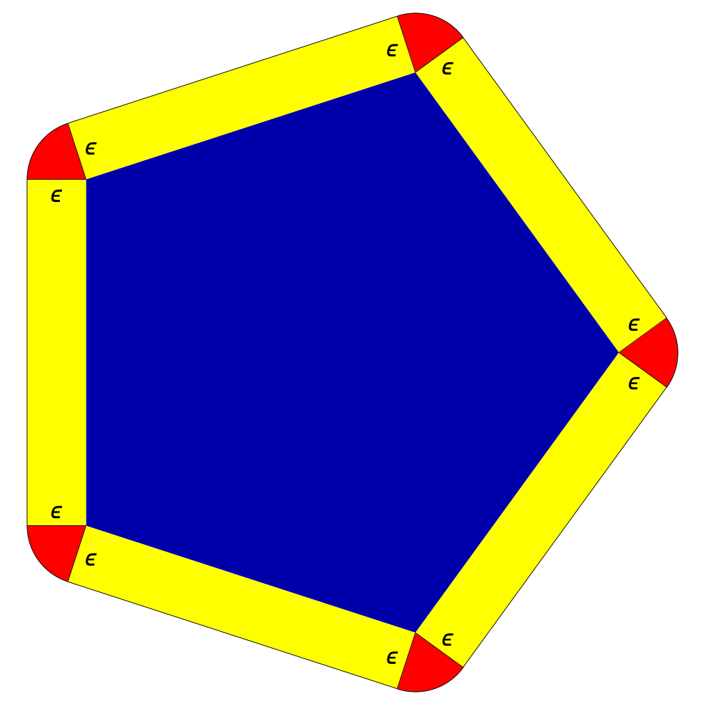
Suppose the slice was a polygon, rather than a smooth curve. If we computed the area of the set of all points that lay outside the polygon within a distance ε, we would find:
A(ε) = p ε + π ε2
where p is the perimeter of the polygon. In the diagram on the right, the polygon is in blue, the regions that contribute to the term p ε are in yellow, and the regions that contribute to the term π ε2 are in red. The reason the red pie-shaped segments add up to exactly one full circle is that the angle each one subtends is the angle between adjacent normals to the sides of the polygon, and since it is convex, these angles are all positive.
The part of this formula that is unaffected by the shape and size of the slice is the quadratic term π ε2, which means the second derivative of the area with respect to ε, evaluated at ε=0, will also be a constant, independent of the shape and size:
A''(0) = 2π

What happens if we look at a shape with a curved boundary and no sharp corners?
The boundary of the blue shape on the right is made from a number of circular arcs, joined together so that their tangents are aligned. The black dots mark the centres of these arcs. Here, the area of the points that lie within a distance ε of the blue shape will be given by:
A(ε) = Σi ½θi ((ri + ε)2 – ri2)
where θi is the angle subtended by each arc, and ri is its radius. The sum of the θi will be 2π, because, as with the polygon, the arcs have to come full circle.
Though the specific values of ri and θi for these arcs appear in the formula for the area itself, if we take the second derivative, we have, once again:
A''(0) = Σi θi = 2π
How can we obtain the same constant as an integral of some quantity over the boundary? The curvature, κ, of a sufficiently differentiable plane curve is the reciprocal of the curve’s local radius of curvature. When the curve itself is simply an arc of a circle with radius ri, the curvature is just:
κi = 1/ri
So if we integrate the curvature along the whole boundary, with respect to arc length s, we obtain:
∫ κ ds = Σi κi si
= Σi (1/ri) ri θi
= Σi θi
= 2π
Although we have performed this calculation for a shape whose boundary consists of a finite number of arcs, the result is true in general for any convex shape whose boundary is a sufficiently differentiable curve.
We can extend this result to a surface integral that evaluates to a constant multiple of the height of the convex body, measured in a specific direction: say, the direction of some unit vector u. We have:
2π h = ∫ κ(u) ds dh
= ∫ κ(u) √(1 – (u · n)2) dS
Here, we write κ(u) to mean the curvature of the curve we obtain by intersecting the surface with a plane orthogonal to u, and the vector n is a local, unit-length normal to the surface. The factor √(1 – (u · n)2) is the sine of the angle between n and u; we need this to account for the varying extent to which an element of the surface with area dS advances in the direction of u.
We can check this formula for a simple case, such as a sphere of radius r, which has h = 2r when measured in any direction. We integrate over the usual spherical polar coordinates θ and φ, and if we set u = (0,0,1) we have:
n = (sin θ cos φ, sin θ sin φ, cos θ)
n · u = cos θ
√(1 – (u · n)2) = sin θ
κ(u) = 1/(r sin θ)
∫ κ(u) √(1 – (u · n)2) dS
= ∫02π ∫0π κ(u) √(1 – (u · n)2) r2 sin θ dθ dφ
= ∫02π ∫0π 1/(r sin θ) sin θ r2 sin θ dθ dφ
= ∫02π ∫0π r sin θ dθ dφ
= 4π r
= 2π (2r)
= 2π h
as required.
So, having reached our goal of finding a surface integral that yields the height in a single direction, given by the vector u, what happens when we average over all possible directions for u?
To deal with this question, we will make use of the fact that the curvature at any point on a surface can be found by approximating it as a suitable quadratic function, which, with an appropriate choice of coordinates, can always be put into the form:
z = a x2 + b y2
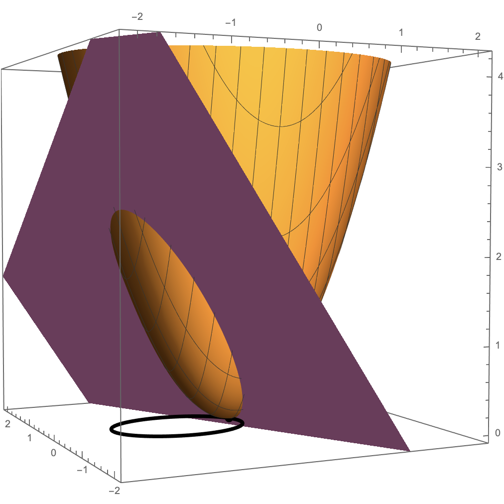
Here, we have placed the origin of the coordinates, (0,0,0), at the point on the surface where we wish to compute the curvature, and we have aligned the axes so that the z-axis is normal to the surface, while the x- and y-axes are oriented to remove any xy term from the quadratic approximation.
The curve formed by the intersection of this surface with the plane through the origin orthogonal to some vector u will generically be an ellipse (as in the image on the right), though it will become a parabola when u points horizontally. [The thick black curve shown here is the projection of the ellipse-of-intersection onto the coordinate plane; we will make use of this shortly.]
There are a number of approaches we might take to compute the curvature of the ellipse-of-intersection, but the simplest is probably to start with the formula for the curvature of a plane curve that is described implicitly by a function F(x, y) = 0:
κF = |Fy2 Fxx – 2 Fx Fy Fxy + Fx2 Fyy| / [Fx2 + Fy2]3/2
The subscripts indicate partial derivatives with respect to x and y. But where does this formula come from?
At any non-singular point on the curve defined by F(x, y) = 0, the gradient of F:
∇F(x, y) = (Fx, Fy)
will be orthogonal to the curve, while the vector rotated 90° from this:
TF(x, y) = (–Fy, Fx)
will be a tangent to the curve. If we move a short distance δ along the tangent, to first order in δ the new gradient is given by:
∇F((x, y) + δ TF(x, y)) = ∇F(x, y) + δ (Fx Fxy – Fy Fxx, Fx Fyy – Fy Fxy)
The particular derivatives multiplied together here come from the chain rule, keeping in mind that when we follow the tangent we are changing the x coordinate by an amount proportional to –Fy, and the y coordinate by an amount proportional to Fx.
Now, we can locate the point of intersection between a line orthogonal to the curve at (x, y), and another line of the same form through (x, y) + δ TF(x, y), by solving the simultaneous linear equations in λ and μ:
(x, y) + λ ∇F(x, y) = (x, y) + δ TF(x, y) + μ ∇F((x, y) + δ TF(x, y));
The solution we get for μ is:
μ = – [Fx2 + Fy2] / [Fy2 Fxx – 2 Fx Fy Fxy + Fx2 Fyy ]
The solution for λ is a little more complicated, but if we then take the limit as δ→0 it becomes the same. And if we multiply the absolute value of this parameter by the length of the gradient vector:
|∇F(x, y)| = [Fx2 + Fy2]1/2
that gives us the distance to the point where these neighbouring lines intersect, in the limit δ→0, which is the local radius of curvature. The curvature given by our original formula is just the reciprocal of that radius.
Now, the ellipse that we get from projecting the ellipse-of-intersection down to the xy plane (the black curve) is given by:
F(x, y) = u · (x, y, a x2 + b y2) = ux x + uy y + uz (a x2 + b y2) = 0
The partial derivatives at x = y = 0 correspond to coefficients of F as a quadratic, doubled for the second derivatives:
Fx = ux
Fy = uy
Fxx = 2 a uz
Fyy = 2 b uz
Fxy = 0
κF = 2 uz (a uy2 + b ux2) / (ux2 + uy2)3/2
The curvature we want is not the curvature of this projected ellipse, but the curvature of the ellipse-of-intersection. So, how are the two related? Because both the plane orthogonal to u and the coordinate plane we are projecting onto contain the tangent to the ellipse-of-intersection at x = y = 0, the projection just rescales the direction orthogonal to the tangent by a factor equal to the cosine of the angle between the planes, which in this case is just uz. So we can recover the curvature of the ellipse-of-intersection by dividing out that factor, to obtain:
κ(u) = 2 (a uy2 + b ux2) / (ux2 + uy2)3/2
If we specify u in polar coordinates, this becomes:
u = (sin θ cos φ, sin θ sin φ, cos θ)
κ(u) = 2 (a sin2 φ + b cos2 φ) / sin θ
Given that the z-axis is normal to the surface, we also have:
√(1 – (u · n)2) = √(1 – cos2 θ) = sin θ
which give us:
2π h = ∫ κ(u) √(1 – (u · n)2) dS
= ∫ 2 (a sin2 φ + b cos2 φ) dS
If we now average this by integrating over the angles for the direction in which we are measuring the height, θ and φ, we have:
2π haverage = 1/(4π) ∫02π ∫0π ∫ 2 (a sin2 φ + b cos2 φ) dS sin θ dθ dφ
= ∫ (a + b) dS
Our two quantities a and b that characterise the shape of the quadratic are half of what are known as the principal curvatures of the surface, while a + b corresponds to their average, known as the mean curvature, which is conventionally denoted by the letter H. If you are wondering where the halves come from, this is essentially because the radius of curvature of a parabola y = ax2 at the origin is 1/(2a), or equivalently, because the quadratic approximation to a circle of radius r sitting on the x-axis at the origin is y = x2/(2r).
So we have the remarkably simple result:
haverage = 1/(2π) ∫ H dS
NB: Don’t confuse the mean curvature, H, with the Gaussian curvature, which is the product of the principal curvatures rather than the average.
Just to check that we aren’t missing any factors, if we look at a sphere of radius r, whose mean curvature is H = 1/r, and whose surface area is 4π r2, this gives us the correct average height of 2r.
This is a nice result for curved surfaces, but what are we to do in the case of polyhedra, where the curvature is zero on the faces and infinite along the edges? It turns out that we can go back to something very similar to our starting point, where we looked at the second derivative of the rate of change of the area of a region within a distance ε of a polygonal slice.
If we compute the volume V(ε) of the region that lies within a distance ε of a convex solid with a smooth surface, we find that:
V''(0) = 2 ∫ H dS = 4π haverage
This is easy to confirm for a sphere:
V(ε) = (4π/3)[(r + ε)3 – r3]
V'(ε) = 4π (r + ε)2
V''(ε) = 8π (r + ε)
V''(0) = 8π r = 4π (2r)
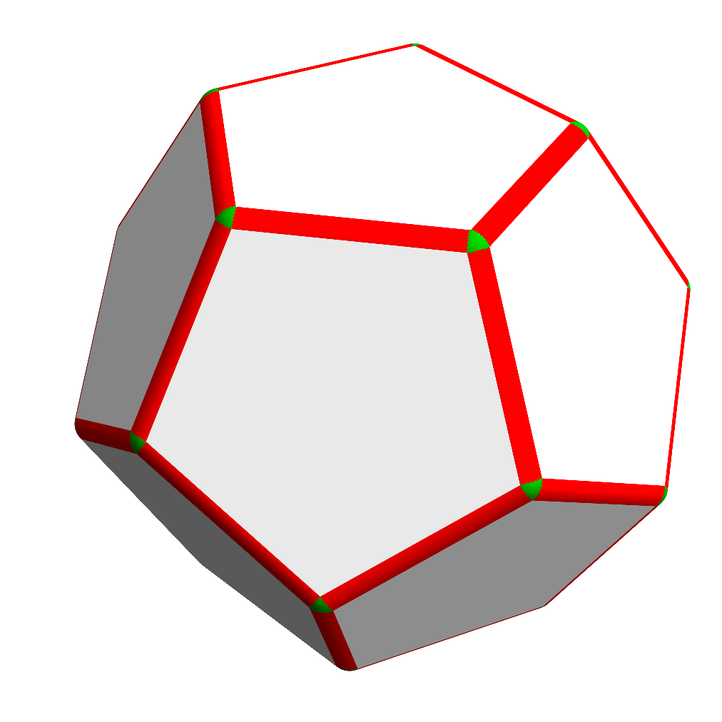
For a polyhedron, like the dodecahedron on the right, we can break the volume V(ε) down into three contributions: those associated with faces (white), edges (red), and vertices (green).
The face-associated volumes are just the product of the face areas and ε, so they are linear in ε and contribute nothing to the second derivative of the volume. And of course the mean curvature is zero on the faces, so this is consistent with our original formula.
The vertex-associated volumes are cubic in ε, so their second derivative is proportional to ε and vanishes once we set ε = 0. If we were approximating the polyhedron by rounding off its vertices, the mean curvature on the segments of spheres at the vertices would be 1/ε, but the surface area would be proportional to ε2, so the contribution from these parts to the surface integral would be proportional to ε, and would tend to zero in the limit of a better approximation.
The edge-associated regions are segments of cylinders with radius ε, so their volumes take the form:
Vi(ε) = ½ei θi ε2
where the ei are the edge lengths, and the θi are the angles of the cylindrical segments; each θi will equal π minus the internal dihedral angle δi between the faces that meet along the edge. Because these terms are quadratic in ε, they have a second derivative that survives when we set ε = 0. And if we were approximating the polyhedron by rounding off its edges, the mean curvature here would be 1/(2ε), while the surface area would be ei θi ε, so the contribution to the surface integral would be independent of ε.
What we are left with, for any polyhedron, is:
V''(0) = Σi ei θi = Σi ei (π – δi)
from which it follows that:
haverage = 1/(4π) Σi ei (π – δi)
We can check this for the unit cube, with 12 identical edges:
ei = 1
δi = π/2
haverage = 1/(4π) Σi ei (π – δi)
= 12/(4π) π/2
= 3/2
in agreement with our previous result using the formula for zonohedra. We can also check this for a prism extruded from a 2n-gon, where the polygonal faces have edge lengths e and the others faces are e × h rectangles. So there are 4n edges of length e with a dihedral angle of π/2, and 2n edges of length h with a dihedral angle of π – π/n.
haverage = 1/(4π) Σi ei (π – δi)
= 1/(4π) [4n e π/2 + 2n h π/n]
= ½(n e + h)
which again matches our previous calculation.
For a regular tetrahedron, which has six equal edges:
δi = acos(1/3)
θi = π – acos(1/3) = acos(–1/3)
haverage = 3/(2π) acos(–1/3) e ≈ 0.91226 e
The basic result we have for convex solids is:
Average orthogonal shadow of any convex solid = ¼ surface area
This arises from two simple facts: the average area of the orthogonal shadow of a flat rectangle is half the area of that rectangle, and for a convex solid, any straight line will intersect the surface exactly twice (or not at all).
For a non-convex solid, a line might intersect the surface more than twice; for example, for a torus it might enter and exit one side of the doughnut, and then enter and exit the opposite side as well.
In the image on the right, we have drawn the shadow of a torus as if it were a translucent shell, so that portions where a light ray would have crossed through the surface four times are darker than those where it would have crossed just twice.
While there is no simple formula that gives the average area of the shadow if it is construed as the total area where the light has met any obstruction, the same argument that leads to the factor of 1/4 in the convex case can be recovered if we count the darker regions here as double their actual area. That is, if we weight each area in the shadow by half the number of surface crossings, the total quantity we obtain by adding up these weighted areas will have an average that again is equal to 1/4 the surface area, even for a non-convex solid.
For the average height of a non-convex solid, there is a work-around that allows us to obtain an exact result. If the solid is connected, then the convex hull and the original solid will both have the same projection onto the z-axis, and hence the same height, in any orientation. We can then apply the formulas we derived in the previous section to the convex hull.
For example, the convex hull of a torus is just a torus with two flat disks glued to the top and bottom, each with a radius equal to that of the major radius of the torus. Since the mean curvature on these disks is zero, we can find the average height by integrating the mean curvature only on the portion of the original torus that lies farther from the axis than the major radius. The result is:
hTorus, average(R,r) = 2r + πR/2
where R, r are the major and minor radii of the torus.