A didicosm is a certain kind of three-dimensional space, one of ten platycosms, the name given by the mathematician John Conway[1] to a space that has a finite volume, no boundary, and a flat geometry: the same geometry locally as ordinary Euclidean space. Four of the ten platycosms are non-orientable (a property for which the Möbius strip is the most famous two-dimensional example) which would lead to serious complications if we lived inside such a space, as it would allow matter to be transformed into its own mirror image just by travelling around a loop. The remaining six, including the didicosm, are potentially candidates for the shape of our own universe, if it happens to be finite.[2] (The didicosm is also referred to as a Hantzsche-Wendt Manifold, named after the mathematicians who discovered it in the 1930s, but we will use the name that Conway gave it much later.)
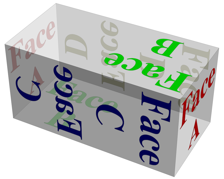
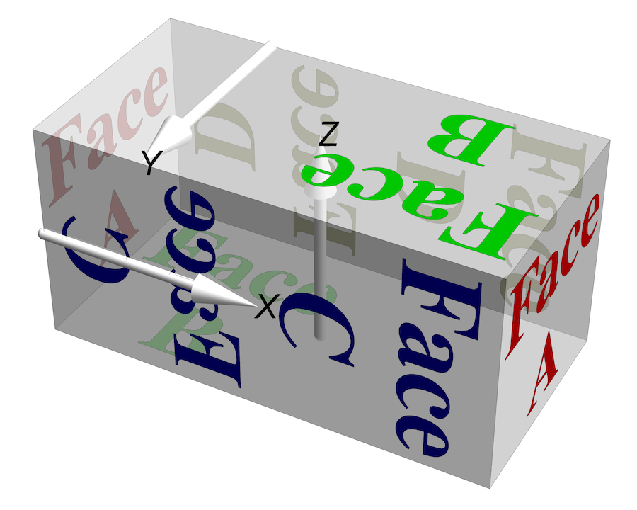
A didicosm can be formed by taking a rectangular prism, as in the image on the right, and “identifying” its faces, so that when you move within the prism to any point on its boundary, you re-enter it at a different point, determined by the way the faces are matched up with each other.
For the two faces labelled Face A this is done in the simplest way possible: if you hit the front Face A, you jump to the corresponding point on the back Face A, and vice versa.
For the two faces labelled Face B, the identification is a little trickier: when you reach points on these faces, you jump to the other face while also undergoing a rotation by 180 degrees around a vertical axis, as indicated by the way the labels are rotated in the image.
For the face labelled Face C, you jump to a new horizontal coordinate by adding or subtracting half the length of the face, while your vertical coordinate is reflected in the horizontal midline of the face. The same thing happens for Face D.
These different instructions might leave you worrying about what happens along the edges, and at the vertices, of the prism. At first sight, the instructions seem to be potentially contradictory. For example, suppose you hit an edge shared by faces labelled Face A and Face B; the instructions for Face A tell you to jump to another point at the same height, while those for Face B tell you to jump between the top and bottom faces. But just as the two faces labelled Face A only comprise a single rectangle within the didicosm itself, the four edges shared between faces labelled Face A and Face B only comprise a single line segment in the didicosm.
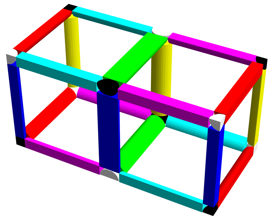
In the image on the left, that single line segment is surrounded by a red cylinder, which is split into quarters in this view, but is a continuous object in the didicosm. The cylinders of various colours here, though they appear divided into halves or quarters, each surround a single line segment and are continuous objects in the didicosm.
Similarly, there are really only two distinct points in the didicosm that correspond to vertices of the rectangular prism, and there are black and white spheres centred on them in this image.
You might also worry that some features on the boundary of the prism will appear in the didicosm as defects in its geometry, preventing it from being locally the same as Euclidean space at some points, or singling out certain places as special. But this is not the case. Just as you can form a perfectly flat version of a torus (the surface of a doughnut) by identifying opposite edges of a square, without causing any irregularity in the geometry, the same thing happens here: every point in a didcosm looks the same as any other, with no trace of the construction from the prism surviving.
Since every path that would take you out of the rectangular prism just leads you back into it somewhere else, the didicosm itself has no boundary. But to be clear, this way of describing the topology of the didicosm should not be taken as implying that it really is a box sitting inside a larger Euclidean space, and some process has connected up its faces in this peculiar fashion. It is simply a handy way for us to visualise how things are connected.
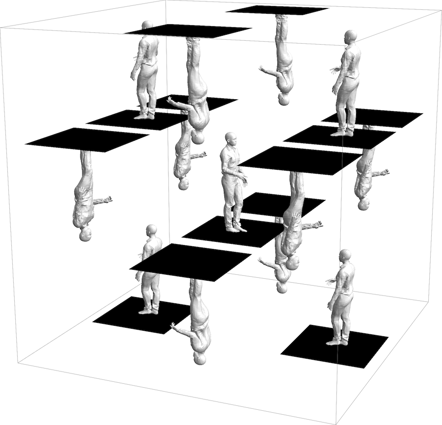
Suppose you were standing inside a didicosm of a fixed size that was small enough for light to cross the whole space in a fraction of a second. (This is in contrast to the situation in cosmology, where the didicosm would be billions of light years across at present, and would also be changing size, having been expanding ever since the Big Bang.) The image on the right shows a small part of what you would see. This “kaleidoscopic” view is formed by gluing extra copies of our original rectangular prism to its six faces, and then further copies to their free faces, and so on; in principal we could fill all of infinite, three-dimensional Euclidean space with copies of the original prism this way.
These copies of the prism are not only shifted relative to the original, they are rotated as necessary to allow their faces to match up correctly. Note that none of the copies are mirror images of the original; the figure’s raised hand is always their right hand.
One way to understand the shape of a space is to study the different kinds of loops that you can draw within it. Suppose you fix a point P in the space, and consider every possible continuous loop you can traverse that starts and ends at P. This will include the loop where you do nothing, and just stay at P, along with loops where you move a short distance away from P and then come back, as well as loops that might cross the whole space one or more times in different directions before returning to P.
That sounds a bit unwieldy, and in a continuous space there will always be an infinite number of loops that are very similar, if you treat the slightest variation in the path you take as giving you a different loop. But we can shift the focus to more interesting properties of the loops, by considering two loops to be equivalent if we can continuously deform one into the other, while keeping their ends fixed at point P. (This kind of continuous deformation of one path into another is known as a homotopy.) You can imagine that the loops are made of some kind of perfectly stretchy, perfectly flexible cord, so their length and shape can be changed as much as you like, and this magical cord can even intersect itself (allowing, say, a figure 8 as a legitimate loop) and pass through itself (so any locally knotted section can be unknotted). The only obstacle to transforming one loop into another comes from the nature of the space itself. The number of possible equivalence classes of loops will be much smaller than the number of loops, though it can still be infinite.
In Euclidean space, or on the surface of a ball, every loop can be continuously deformed into one that just stays at P (the so-called trivial loop). But on a torus (the surface of a doughnut), loops that wind a different number of times around the torus will belong to different equivalence classes. In fact, we can classify all the equivalence classes with a pair of integers, (a, b), that count how many times the loop winds around the torus in each of two directions, with positive or negative integers depending on the direction we took.
The easiest way to picture this is not by drawing a three-dimensional doughnut and looking at its surface, or by drawing a single square whose opposite edges are identified, but by taking a kaleidoscopic view of the torus, where we fill up two-dimensional Euclidean space with copies of the square that represents the torus.
The image on the left shows some loops in the equivalence class of all loops that travel twice around the torus in one direction, and once in the other direction, so we classify it as the (2,1) class of loops. In the kaleidoscopic view, we can simply draw an arrow that travels the chosen number of squares from the base point P in the original square to another copy of P. We then translate the pieces of the arrow that lie in other squares back to the original. This approach automatically satisfies the need for any path that leaves the square along one edge to re-enter it at the corresponding position on the opposite edge. (Here, we have also replicated everything in all of the squares.)
This example also shows that if we take a (2,0) loop that goes twice around the torus to the right in this diagram, and then follow it with a (0,1) loop that goes once around the torus in the upwards direction, the loop we get by joining those loops can be deformed into the one we get by first doing a (0,1) loop and then a (2,0) loop. That might seem too obvious to be worth mentioning, but there are other spaces where the same kind of rule doesn’t hold: combining the same two loops in a different order can yield different equivalence classes for the combined loop.
In general, the equivalence classes of loops that start and end at a chosen point in a space form what is known as the fundamental group of the space (also called the first homotopy group). A group in mathematics refers to a set of objects and an operation that takes two of them and yields another; for example, the positive real numbers can form a group with the operation of multiplication. A group also needs an identity: an object that leaves other objects unchanged, like the number 1 leaves numbers unchanged under multiplication, and an inverse for every object, which acts like the reciprocal of a number.
In the fundamental group, the operation on equivalence classes of loops comes from joining two loops together. If X and Y are two equivalence classes of loops, we can pick any loops in these classes, follow one from P to P, and then the other from P to P, and the combined loop will also take us from P to P. We write the equivalence class of that combined loop as X Y, and we will adopt the convention that the rightmost loop, the one in Y, is the one we follow first. It is important to note that after joining the two loops, creating a combined loop that passes through P halfway through the journey (as well as starting and ending at P), we do not need to hold the midpoint fixed at P when we go on to make the whole equivalence class by deforming that loop. You can see this in the animation of the (2,1) equivalence class, where two of the specific loops pass through a third copy of P, but most of them only start and end at copies of P.
In the fundamental group, the identity is the equivalence class of the trivial loop, where we start at P and just stay there. The inverse of any equivalence class is found by taking one of its loops and travelling around it in the opposite direction. If you follow any loop from P to P with the same loop traversed in the opposite direction, it is not hard to see that you can deform the combined loop into one that simply stays put at P.
For the torus, the group we get by acting on the equivalence classes of loops this way is isomorphic to the group we get by taking pairs of integers and adding them as the group operation, by which we mean that we can identify all the elements of one group with all the elements of the other, and all the group operations will yield the same results. We say:
The fundamental group of the torus is ℤ × ℤ.
where ℤ is the symbol mathematicians use for the set of all integers, and × here refers to the Cartesian product, which just means taking pairs of things from the sets we have combined this way. So, we are restating the claim we made earlier, that the equivalence classes of loops on the torus can be classified by pairs of integers, (a, b), but we are also saying that the group operations are:
(c, d) (a, b) = (a+c, b+d)
(a, b)–1 = (–a, –b)
Having seen how things work for a two-dimensional torus, it will probably be no surprise to learn that for a three-dimensional torus — the platycosm you get by identifying all three pairs of opposite faces of a rectangular prism in the simplest possible way — the fundamental group is just ℤ × ℤ × ℤ, the set of all triples of integers, with addition as the group operation again. (Conway calls this kind of space a “torocosm,” but most people call it a 3-torus.)
The didicosm has a different fundamental group than the 3-torus, but we can find it by examining the kaleidoscopic view we have already created. In the case of the 2D torus, the identification of each square in the kaleidoscopic view with a pair of integers seemed like an obvious choice, but we need to step back and think about this a bit more carefully. When we consider a loop within the space itself, we get an arrow in the kaleidoscope, starting at one copy of P and ending at another. We can classify these arrows by the number of squares they cross in each direction, and this pair of integers gives us a recipe that we can use to copy any square into any other square, purely by shifting it to a new location — a geometrical operation that mathematicians call a translation.
But for the kaleidoscopic view of the didicosm, we need rotations as well as translations. It turns out that all the possible ways of copying the original prism can be generated by some combination of three “screw rotations”: translations along certain axes combined with rotations around those axes.
The image on the right shows the axes of the three screw rotations as the white arrows labelled X, Y and Z, with the length of the arrow giving the distance by which we translate. In each case, the rotation is by 180 degrees around the axis.
The screw rotation we have called X, and its inverse X–1, take the two copies of the Face C label into each other. The screw rotation Z, and its inverse Z–1, do the same for the Face B labels. The screw rotation X repeated twice, written X2, and its inverse X–2, do the job for the Face A labels. And for the Face D labels, we can use Z–1 Y and Y–1 Z, where we perform the rightmost operation first.
If we look carefully for algebraic relations between these three screw rotations, we find:
X = Y2 X Y2
Y = X2 Y X2
X Y Z = 1
where by 1 we mean the transformation that does nothing, which is the identity in the group of rotations and translations.
These three equations comprise what is known as a group presentation for the complete set of transformations that give us the kaleidoscopic view of the didicosm. Though it is not as simple and concrete as talking about something like pairs of integers, as we could with the torus, it is enough to pin down all the algebraic properties of this group. What it is saying is that the group consists of any product of powers of any of the two elements X and Y subject to the fact that we can make the substitutions that these equations permit. We don’t need to include Z, because the last equation lets us rewrite Z as Y–1 X–1.
The fundamental group of the didicosm — a group of equivalence classes of loops — is isomorphic to the group of geometrical transformations that give us the kaleidoscopic view, with any loop being identified with the transformation that takes the original base point P to the copy of P where the loop ends up, in the kaleidoscopic view.
In the animation on the left, we convert the equation Y = X2 Y X2, which we originally found for screw rotations, into a homotopy between loops. First, we create a loop by going around the X loop twice (red then green), the Y loop once (blue), then the X loop twice again (cyan then magenta). Then we deform that combination of five loops into a loop that is simply the Y loop.
Despite the presence of equations like this in the group presentation, which sometimes let us replace a complicated loop with a much simpler one, it is not hard to see that the fundamental group of the didicosm is still infinite. For example, all the integer powers of any single one of the generators, X or Y, will be distinct.
There is a sense in which the two kinds of loops that go around a torus exactly once in each of the two possible directions indicate the presence of two different “holes.” If we think of a torus as the two-dimensional surface of a three-dimensional doughnut — say by coating the doughnut with icing and then removing the doughnut itself — then going around the torus the long way takes you around the ordinary hole in the doughnut, while going around the short way takes you around the hollow space where the doughnut used to be.
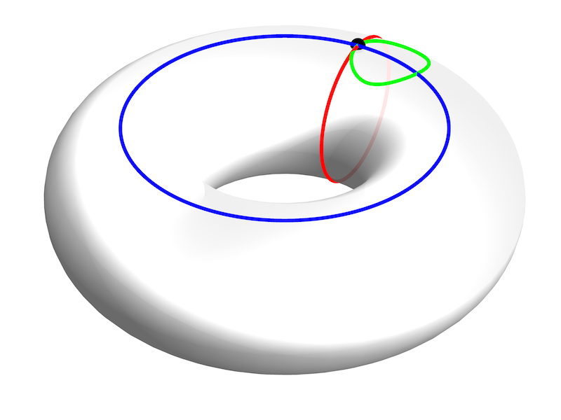
In the image on the right, the blue and red loops circle those two kinds of holes, whereas the green loop does not circle a hole, it just circles a portion of the torus itself.
But spaces in mathematics and cosmology are not generally sitting inside any particular larger space this way. If we want to discuss the intrinsic properties of a space — which are completely independent of any embedding — can we still talk about “holes” of the kind we have described for the torus?
Here is one possibility: the green loop we drew on the torus is the boundary of a region within the torus, whereas the blue and red loops are not. So we could use the existence of a loop that is not the boundary of any region as an indicator of a “hole.” This is similar to the idea that the fundamental group contains loops that can’t be deformed into the trivial loop, and for our example on the torus it more or less matches up with it, but as we will see it is not exactly the same in general.
The mathematics that makes the notion of “loops that aren’t boundaries” precise is known as homology theory. The details of homology theory can be set up in all kinds of different ways, but for our purposes we will focus on a version known as simplicial homology. Don’t be put off by the terminology: a simplex is just a point, a line segment, a triangle, a tetrahedron, or the analogous geometrical object in any higher dimension. An n-simplex is an n-dimensional set, so a triangle is a 2-simplex, a line segment is a 1-simplex, and a tetrahedron is a 3-simplex. When we are talking about Euclidean geometry, an n-simplex is the convex hull of its set of n+1 vertices: the smallest convex set that contains those vertices.
When we study an n-dimensional space using simplicial homology, first we need to chop it up into n-simplices. In the case of a 2-dimensional space that means dividing it into triangles, but the term triangulation is often used, for any number of dimensions, to mean a division into n-simplices.
Having divided our space into n-simplices, that also gives us a whole lot of simplices of lower dimension, all the way down to 0-simplices, or points. For example, each tetrahedron into which we have divided a 3-dimensional space will have four triangular faces, each of which has three line segments as its edges, each of which has two vertices as its endpoints. Of course many of these lower-dimensional simplices will be shared between the higher-dimensional ones, so we need to make sure that we only count them once.
If we assign numbers (any way we like) to all the individual vertices, that gives us a way of deciding when a list of vertices in any of our n-simplices is in ascending order, and we will use that to assign unambiguous descriptions to all of them.
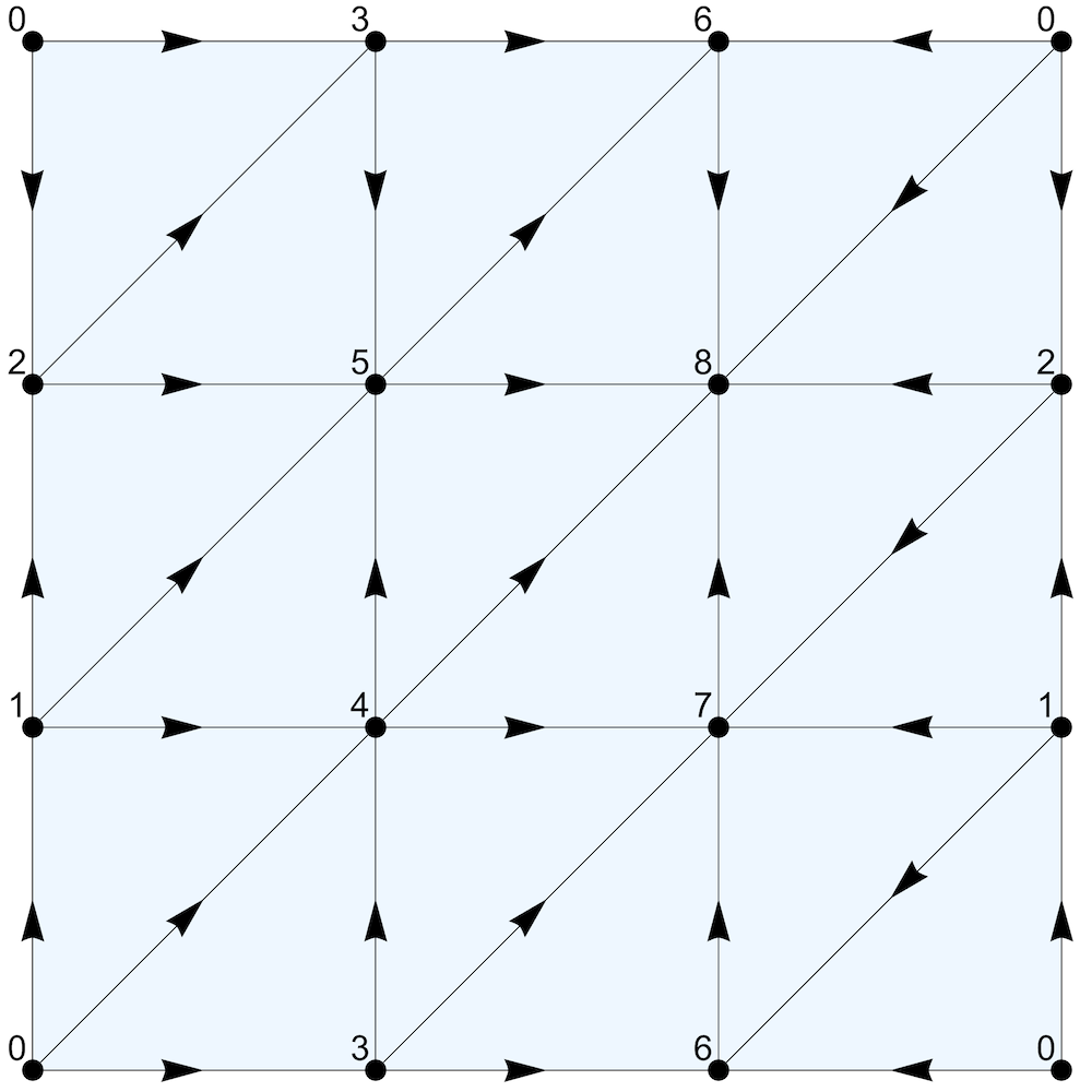
For example, in the image on the left, we have triangulated a torus (as a square with opposite edges identified) into 18 triangles, and we have numbered the nine vertices 0 to 8. This then allows us to label the 27 edges by their two vertices in ascending order: e.g. [2 5], [4 7] etc.; in the diagram, we have drawn an arrow on each edge from the lower-numbered vertex to the higher. And the 18 triangles can also be labelled by listing their vertices in ascending order: e.g. [4 5 8], [1 6 7] etc.
The goal in homology theory is to construct groups (in the mathematical sense) that make all our concepts amenable to studying with the tools of abstract algebra, just as we did with the equivalence classes of loops in the previous section. To that end, in simplicial homology we start by constructing groups for all the k-simplices in our triangulated space, where k goes from 0, for the vertices, up to n, the dimension of the space itself.
Each such group, which we will call Ck for k = 0, 1, ... n, has as its elements all possible “formal sums” of k-simplices in the triangulation multiplied by arbitrary integer coefficients, or weights. For example, any element of C0 for our triangulation of the torus will look like:
c0 [0] + c1 [1] + ... + c8 [8]
where the cv are any integers, and [0] ... [8] are labels for the vertices. Similarly, the elements of C1 are sums of integer multiples of the 27 edges, [0 1] ... [7 8], and the elements of C2 are sums of integer multiples of the 18 triangles, [0 1 4] ... [5 6 8].
The group operation on these Ck is addition of these sums, which amounts to adding the weights for each k-simplex; the identity is the empty sum, and we obtain an inverse by negating all the weights. These groups are obviously commutative, aka abelian: it makes no difference which element comes first and which comes second when you add them. In fact, these groups are all isomorphic to ℤ × ℤ × ... ℤ, the Cartesian product of as many copies of the integers as there are k-simplices in the triangulation.
The next ingredient in simplicial homology formalises the notion of taking the boundary of a simplex. If we look at a triangle, say [0 1 4], it is not hard to see that we can obtain all the line segments on its boundary just by dropping each of the 3 vertices in turn from the list for the triangle, and leaving the remaining ones to describe the edge; this gives us [1 4], [0 4] and [0 1].
It turns out to be extremely useful to add a small twist to this process: we write the boundary we obtain this way as a formal sum of the edges, but we alternate between the signs we give them. So we will say:
Boundary of triangle [0 1 4] = [1 4] – [0 4] + [0 1]
Why is this useful? Because if we apply the same recipe to the formal sum of the edges, we get:
Boundary of edge [1 4] = [4] – [1]
Boundary of edge [0 4] = [4] – [0]
Boundary of edge [0 1] = [1] – [0]
Boundary of (Boundary of triangle [0 1 4]) = ([4] – [1]) – ([4] – [0]) + ([1] – [0]) = 0
This lets us capture the basic notion in topology that the boundary of a set has no boundary itself; e.g. the boundary of a triangle or a disk forms a closed loop with no endpoints.
If we take the boundaries of everything in Ck+1, we will get a set of elements of Ck that are all closed loops, or similar objects of other dimensions, such as closed surfaces. Certainly, none of them will have any boundaries themselves. We will call this set Bk; it contains all the formal sums of k-simplices that correspond to the boundary of something of the next-highest dimension.
Bk = the boundaries of everything in Ck+1
Because of the way we have defined our groups, and the boundary operation, each Bk will be a group as well, a subgroup of Ck. In this context, that means that we can add elements of Bk and take their inverses, and the result will always still be in Bk. Also the group identity, 0, of Ck, is also in Bk, since it is formally the “boundary” of 0 in Ck+1.
Now, while Bk contains all the boundaries of all formal sums of (k+1)-simplices, and the way we have defined things, we know for sure that all the boundaries of elements of Bk are zero, the converse need not be true. That is, there might be sums of k-simplices in Ck whose boundaries are zero, but which do not lie in Bk. That is, they are closed loops (or closed surfaces, etc.) or sums of such things, that do not correspond to the boundary of any higher-dimensional element. This is precisely the notion that we set out to capture.
For example, consider the element of C1 in our triangulation of the torus:
y = [3 4] + [4 5] – [3 5]
Boundary of y = [4] – [3] + [5] – [4] – [5] + [3] = 0
The element y is not in B1; it cannot be created as the boundary of anything in C2.
We will give the name Kk to all the elements of Ck whose boundaries are zero. [In mathematical terminology, Kk is the kernel of the boundary homorphism from Ck to Ck–1.] It probably won’t surprise you to learn that Kk is a subgroup of Ck, and Bk in turn is a subgroup of Kk.
Now, we could just ask the question: what elements, if any, are left in Kk if we remove all the elements of Bk? That would give one description of the phenomenon we are seeking to describe. But it turns out to be more useful to do something that is very common in group theory, when we have a normal subgroup sitting inside a group and we want to compare the two groups. You can follow the link if you want to know the definition of this in general, but for abelian groups, all subgroups are normal, and it will be easy to see that the construction we are about to perform works in this particular case. Instead of removing elements of the subgroup from the larger group, we “factor out” the subgroup, effectively treating all of its elements as being the identity of a new group, called the factor group (aka quotient group).
A simple example of forming a factor group is to take the integers ℤ under addition, and use the subgroup of, say, all multiples of 7, which we can write as 7ℤ. The factor group, ℤ/(7ℤ), is a new group where we treat all multiples of 7 as being zero, and addition is performed modulo 7; we write this as ℤ7. Effectively, we have sliced up ℤ into 7 shifted copies of 7ℤ, and called them 0,1,2,...6 according to the amount we have added to them, to create our new factor group with just 7 elements. In group theory, when we slice up a group into copies of a subgroup, the copies are known as cosets, and when the subgroup is a normal subgroup, the cosets themselves form a group.
In simplicial homology, our final goal is to construct the factor groups:
Hk = Kk / Bk
These Hk are what are known as the homology groups of our space. Specifically, the first homology group, H1, tells us to what extent there are closed loops in the space that are not boundaries of two-dimensional regions. If all closed loops were the boundaries of regions, then we would have B1 = K1, i.e. we would be setting all of K1 to the identity, 0, when we formed the factor group, and H1 would be the trivial group, {0}. For the surface of a sphere or the Euclidean plane, that is exactly what happens: both the fundamental group and the first homology group are trivial.
Sometimes there is a relatively simple way to construct the first homology group, H1, without calculating B1 or K1. If we already know the fundamental group of the space, we can just “abelianise” it. As we mentioned earlier, an abelian group is a group where the order in which you perform the group operation makes no difference. This relationship between the first homology group and the first homotopy group is one of the results of the Hurewicz theorem.
In the case of the torus, the first homology group is ℤ × ℤ: the same as the fundamental group, since the fundamental group is already abelian. What this means is that there is a distinct copy of B1 inside K1 corresponding to every pair of integers, which in turn corresponds to adding arbitrary integer multiples of the two different loops that cross the full width of the torus to each of the elements of B1.
We can find the first homology group for the didicosm by taking the equations from our group presentation for the fundamental group, and adding the rule that we can reorder any of the terms.
So, in the first homology group we have:
X = Y2 X Y2 = Y4 X
Y4 = 1
Y = X2 Y X2 = X4 Y
X4 = 1
This tells us that the entire first homology group is generated by two elements, X and Y, and we only need to include their powers from 0 to 3. In other words, the group contains just 16 elements, which are essentially the same as pairs of integers (a, b), where a and b belong to the set {0,1,2,3} and correspond to the powers of X and Y. The group operation is addition modulo 4. We say:
The first homology group of the didicosm is ℤ4 × ℤ4.
It can be shown that any abelian group generated by a finite number of elements is equivalent to a Cartesian product of a certain number of copies of the full set of integers, and a finite part like this — the Cartesian product of a number of copies of ℤr for various values of r — though either ingredient can be missing. As we have noted, the first homology group of the torus is ℤ × ℤ, and there is no finite part. But in the case of the didicosm, there are no copies of ℤ, just the finite part we have described.
What this means, when we think back to our definition of the first homology group as:
H1 = K1 / B1
is that B1 is not all of K1, but nor is K1 higher-dimensional than B1 in the way it is for the torus. Rather, there are exactly 16 copies of B1 in K1, and we obtain them by adding terms of the form:
a X + b Y
to each of the elements of B1, where a and b are integers from the set ℤ4 = {0,1,2,3}, and by X and Y we mean elements of C1 (that is, sums of edges in our triangulation) that correspond to the equivalence classes of loops, X and Y, that we originally encountered in the fundamental group of the didicosm. You might object that in our triangulation of the didicosm there could be many different elements of C1 that belong to the same equivalence classes, but they will all differ from each other by elements of B1, so it makes no difference which ones we choose to add to the whole subgroup B1.
This poses the following puzzle: traversing a loop from the equivalence class X in the fundamental group 4 times in a row does not produce a loop that we can deform into a trivial loop; in the fundamental group X4 ≠ 1. But the first homology group is telling us that any multiple of 4 times any corresponding element of C1 must lie in B1, which means it is the result of taking the boundary of some sum of triangles in C2.
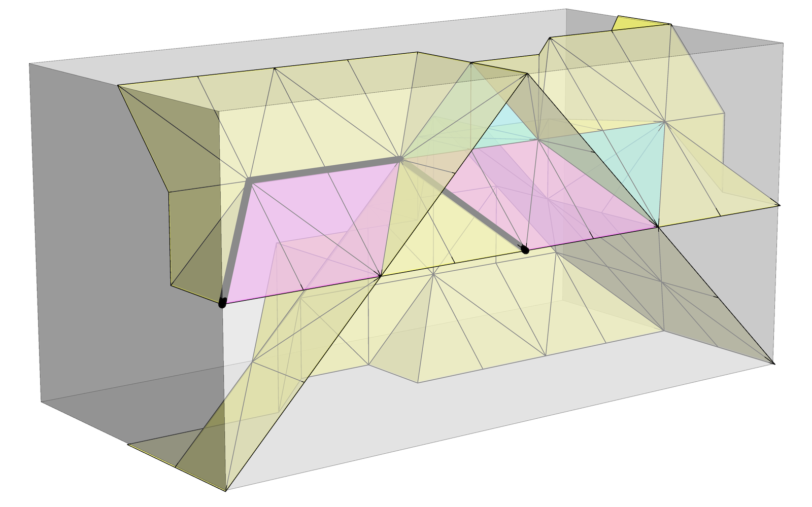
The image on the right shows one solution found from a triangulation of the didicosm. Here, the thick black line represents the loop X4, while the triangles have been coloured to show various integer weights: yellow=±1, cyan=±2, magenta=±3.
Note that the thick black line is always an edge to one yellow and one magenta triangle, allowing the total value of the boundary to reach 1 + 3 = 4 all along its length. All other edges are shared either by two triangles of the same absolute weight, which give equal but opposite weights that cancel out along their shared boundary, or multiple triangles that give the boundary a total weight of zero, like 1 + 1 – 2 = 0, 1 + 2 – 3 = 0, or 1 + 1 + 1 – 3 = 0.
So, there is a sense in which X4 does arise as a boundary, without being contractible to a trivial loop. And the reason this is true for X4 but not any lower power of X is that the weights on the triangles cannot be made any smaller: the yellow ones are already just 1, so if we tried to divide everything by 4 we would be left with fractional weights for some surfaces.
We found this solution with algebraic methods, but we could convert it into an actual surface immersed in the didicosm: that is, a surface mapped into the space in such a way that different portions of the surface end up overlapping with each other, in contrast to an embedding, where no parts of the mapped surface intersect. (Klein’s bottle famously cannot be embedded in three-dimensional Euclidean space, but can be immersed.)
To construct this surface as a topological space S outside the didicosm, we can treat each triangle in the solution as being mapped from as many different triangles in S as the absolute value of the triangle’s weight, so while the yellow triangles here would come from single triangles in S, each cyan triangle would come from two different triangles, and each magenta triangle from three. We can then join up these triangles in S to others that are mapped to their neighbours in the didicosm, while ensuring that S has a single circle as its boundary, which is mapped in the didicosm to a curve that traverses the X loop four times.
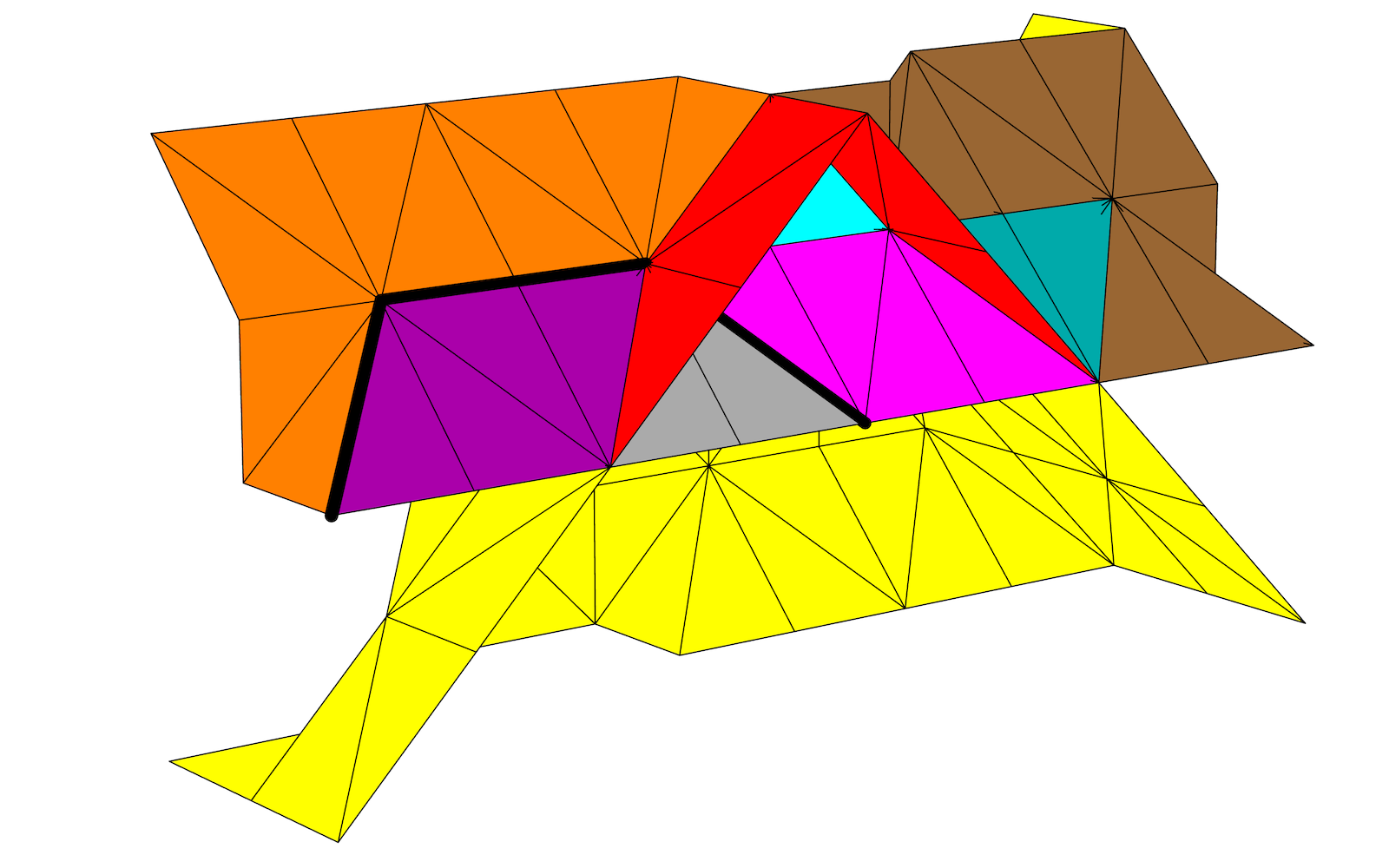
In the image on the left, we have split up the regions of equal weight into pieces that we can draw in the plane as (topologically, but not geometrically, equivalent) polygons with some identifications between pieces of their boundaries.

In the image above, we show these polygons in the plane. Here the vertex numbers come from the original triangulation of the didicosm, and are just arbitrary labels, but they let us match up edges with the correct orientation. The lower-case letters a-i mark edges that are shared by just 2 regions of the same weight in the triangulation, while the upper-case letters A-G mark edges that are shared by 3 or 4 different regions, so we have some choice as to how the associated polygons in the surface S join up.
The edges marked with heavy black lines lie on the boundary that we wish to traverse 4 times in a single loop.
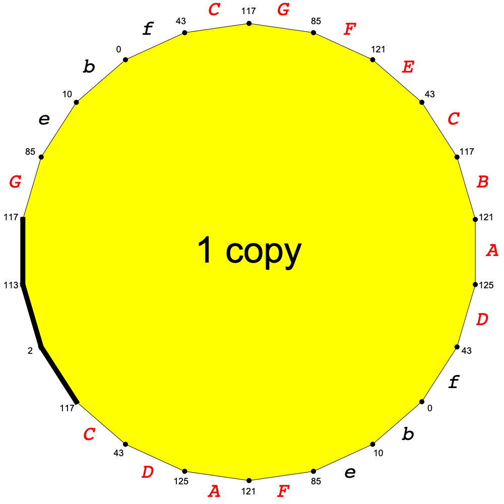
If we glue all the weight-1 pieces together, we get the polygon shown on the left. The pairs of edges marked e, b, f are identified with each other, with no choices to be made.
The two weight-3 (magenta) pieces fit together in the obvious way, along the edge i, to form a hexagon with three edges on the boundary loop, along with gluable edges C, E, B. So we are then left to fit together 3 copies of that magenta hexagon, 2 copies of each of the cyan triangles with edges A, D, E and G, F, B, and the single yellow polygon shown on the left.
Since there is one edge marked C on each magenta hexagon, and three edges marked C on the yellow polygon, we can glue all three hexagons onto the polygon along those edges.
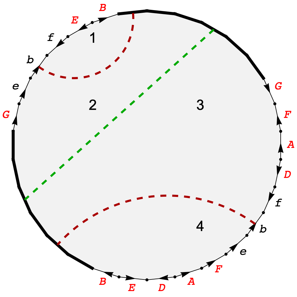
We then have some choices as to where we glue the 4 cyan triangles, but one set of choices gives us the polygon on the right as a final representation of the whole surface, S. Here, all labelled edges come in pairs that are identified with the arrows pointing in the same direction. The heavy black line corresponds to four traversals of the X loop in the didicosm, but here it is a single continuous loop that forms the boundary of the surface.
In terms of their topology, all surfaces can be fully classified if we know three things about them:
We can tell that this surface is non-orientable, because we can embed a Möbius strip in it, e.g. by taking a strip of the surface that starts and ends on the edge labelled E.
We can check that this surface has a single boundary component by noting that both of the heavy black boundary lines start and end at the same two points: the start of edge G and the end of edge B.
To determine the rank, note that the red and green dashed lines start and end on the boundary (with an apparent jump in the red case where it hits a non-boundary edge of the polygon), and they clearly do not intersect. But do they divide the surface S, or not?
They divide the polygon into 4 regions, which we have labelled 1 to 4. But all 4 regions are connected:
So we can move continuously between any two points on S without crossing these dashed lines. That means the rank of S is 2.
These three properties of S show that it is topologically the same as Klein’s bottle with a disk removed!
We can double-check that we have the rank correct by calculating the Euler characteristic of the surface we get if we glue a single disk to the boundary of S. The Euler characteristic, usually written as χ (the lower-case Greek letter chi), is given by the formula:
χ = V – E + F
where V, E, F count the number of vertices, edges and faces in a division of the surface into polygons. If we treat the disk we glue to the boundary along the two heavy black lines as a polygon with two edges and two vertices, then it is easy to see that we have F=2, and E=11 (the two heavy black lines, plus the nine labelled edges b, e, f, A, B, D, E, F, G).
We need to be careful counting the vertices, as some are shared by two edges and some by three. There are 9 vertices, with the edges that share them as follows:
So, we have:
χ = 9 – 11 + 2 = 0
Klein’s bottle is known to have a Euler characteristic of 0.
The Euler characteristic of a surface with no boundary and the rank of the surface obtained if we remove a single disk from it are related by the formula:[4]
χ = 2 – rank
So our two ways of calculating χ are consistent with the surface having rank 2.
[1] “Describing the platycosms” by J. H. Conway and J. P. Rossetti. (2003). Online at arXiv.org.
[2] “The Hantzsche-Wendt Manifold in Cosmic Topology” by R. Aurich and S. Lustig. Classical and Quantum Gravity Vol. 31 Number 16 (2014). Online at arXiv.org.
[3] “On the coverings of the Hantzsche-Wendt Manifold” by G. Chelnokov and A. Mednykh. Tohoku Mathematical Journal (2) 74(2): 313-327 (2022). Online at arXiv.org.
[4] How Surfaces Intersect in Space by J. Scott Carter. World Scientific, Singapore, 1993.